n <- 10000
df_sim <- tibble(
x1 = rnorm(n, mean = 3.13), x2 = rnorm(n, sd = 0.4),
y = 2 + .2 * x1 + .4 * x2 + rnorm(n)
)
df_fake <- df_sim |>
mutate(x2 = 0.5 * x1 + 0.5 * x2 + rnorm(n, sd = 0.1))
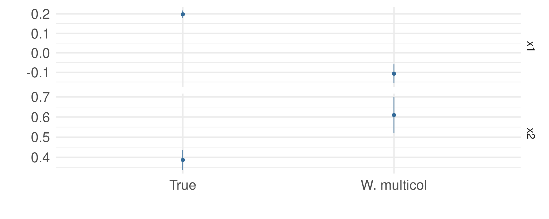
cor(df_fake$x1, df_fake$x2)[1] 0.9118169
Large N & Leeuwenhoek (70700173)
Why should we use multiple regressions, and why controls?

One observes a set of covariates that is, after statistical adjustment, sufficient to make treatment status as-if random.—Keele et al. 2020
\[X_{2i} = \hat\delta_0 + \hat\delta_1X_{1i} + \hat r_{1i}.\]
When cov(X1, X2) = 1, r1i = 0, then \(\hat\beta_1 = \frac{\sum\hat r_{1i}y_i}{\hat r_{1i}^2}\) cannot be estimated.
E.g., \(X_{2i} = 1 + 2X_{1i}.\)
\[\begin{align} Y_i =& \hat\beta_0 + \hat\beta_1X_{1} + \hat\beta_2X_{2} + \hat \epsilon, \text{(PRF)}\\ =& \hat\beta_0 + \hat\beta_1X_{1} + \hat\beta_2(1 + 2X_1) + \hat \epsilon, \\ =& (\hat\beta_0 + \hat\beta_2) + (\hat\beta_1 + 2\hat\beta_2)X_1 + \hat \epsilon,\\ \Rightarrow Y_i =& \tilde\beta_0 + \tilde\beta_1X_{1} + \hat \epsilon. \end{align}\]
Example
\[X = \begin{bmatrix} 1 & 0.99 \\ 0.99 & 1 \end{bmatrix}, \tilde X = \begin{bmatrix} 1 & 0.99 \\ 0.99 & 1.01 \end{bmatrix} \Rightarrow X^{-1} \approx \begin{bmatrix} 50.25 & -49.75 \\ -49.75 & 50.25 \end{bmatrix}, \tilde X^{-1} \approx \begin{bmatrix} 33.44 & 0.3311 \\ 0.3311 & 33.78 \end{bmatrix}\]
E.g., \(X'_2 = 0.5X_1 + 0.5X_2 + \nu.\)
Variance Inflation Factors (VIF, [1, +∞]): A measure of how much the variance of the estimated coefficient βx is “inflated” by the correlation among the predictor variables.
\[VIF = \frac{1}{1 - {R}^{2}_{X_i}} = \frac{1}{Tolerance}\]
\[\begin{align} var(\hat\beta|X) =& \frac{\sum(X_i - \bar X)^2}{[\sum(X_i - \bar X)^2]^2}\sigma_i^2.\\ H_0: var(\hat\beta|X) =& \sum(X_i - \bar X)^2;\\ \Leftrightarrow\frac{\sum(X_i - \bar X)^2}{[\sum(X_i - \bar X)^2]^2}\sigma_i^2 =& \frac{\sigma^2}{\sum(X_i - \bar X)^2},\\ \sum(X_i - \bar X)^2\frac{\sigma_i^2}{\sigma^2} =& \sum(X_i - \bar X)^2 \end{align}\]
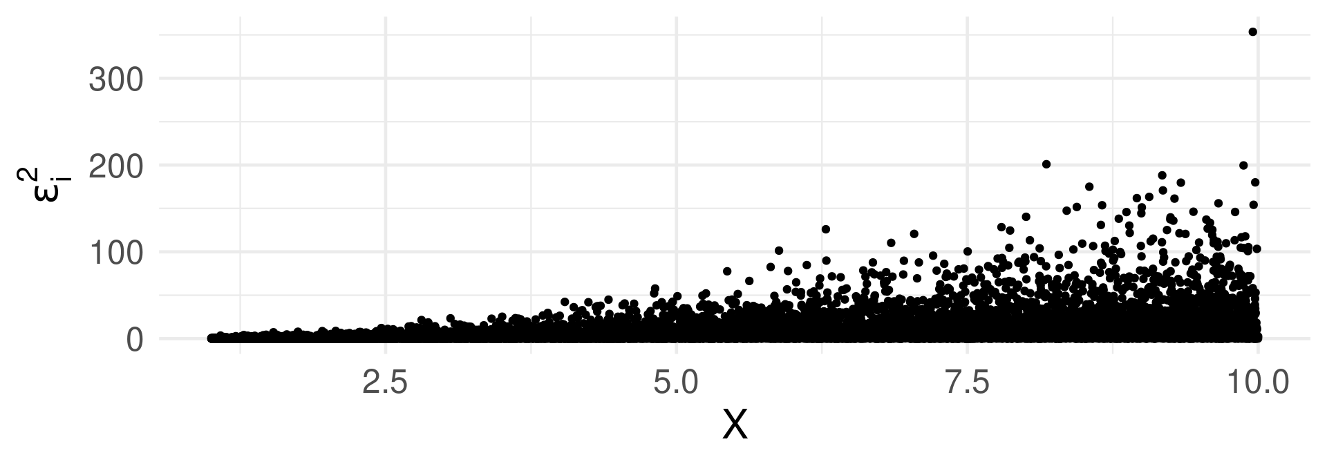
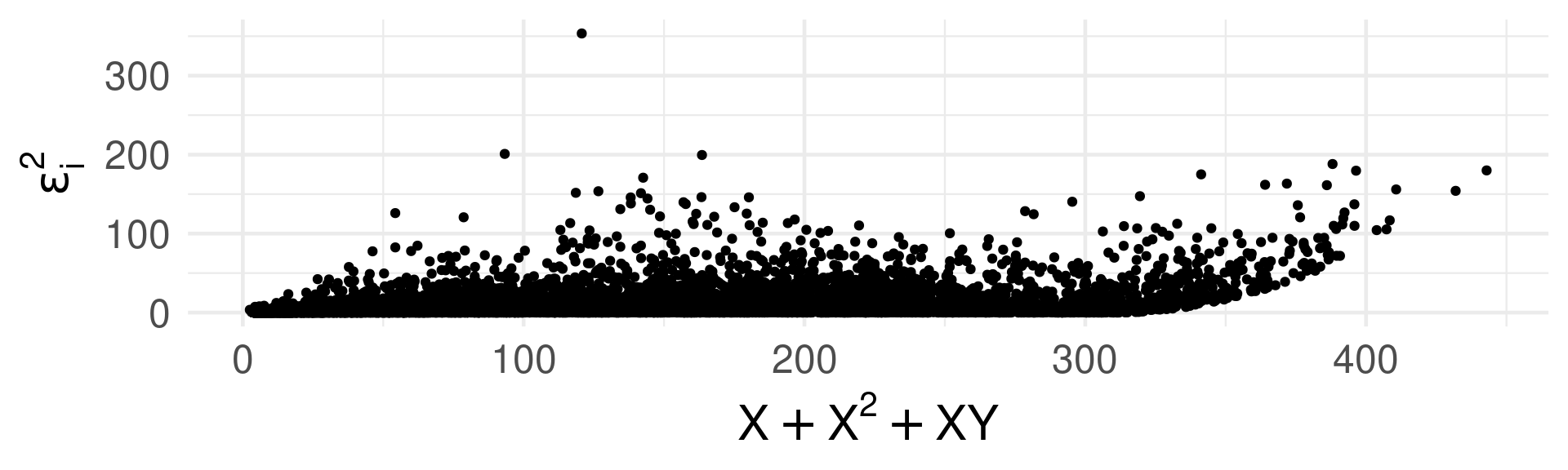
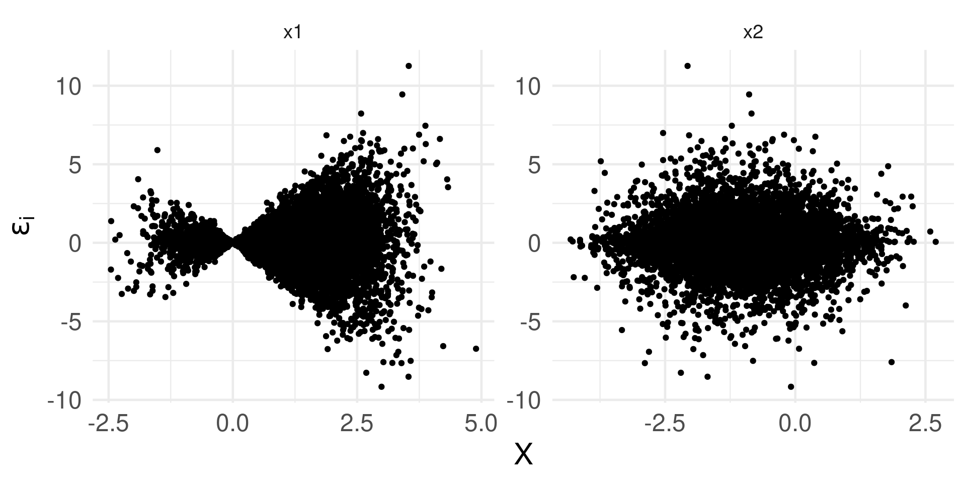
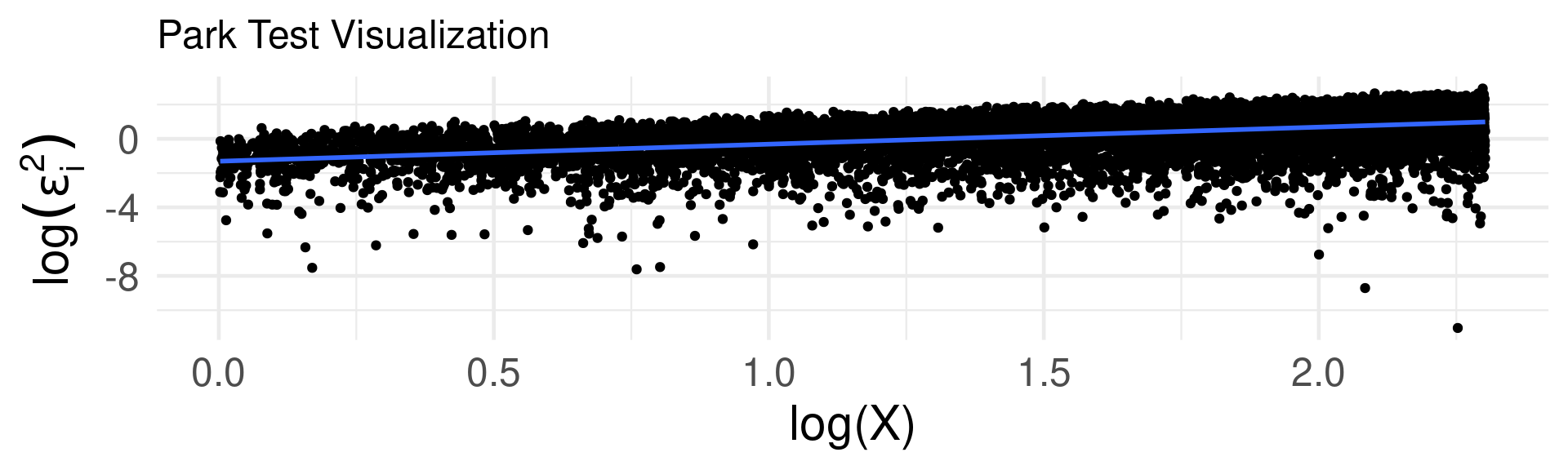
Ocular-inspection test: Use the scalar points of \(\hat \epsilon_i^2\) against \(X_i\)1
Regress \(ln(\hat \epsilon_i^2)\) on some \(X_{ki}\): \[ln(\hat \epsilon_i) = \hat\delta_0 + \hat\delta_1ln(X_{ki}) + \hat\gamma_i.\]
Do the t-test of coefficient in \(ln(X_i)\): \(H_0: \hat\delta_1 = 0.\)
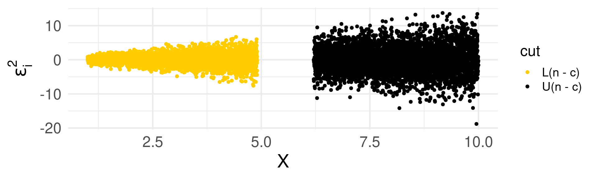
Goldfeld-Quandt test
data: m_fit
GQ = 9.0616, df1 = 4997, df2 = 4997, p-value < 2.2e-16
alternative hypothesis: variance increases from segment 1 to 2
Goldfeld-Quandt test
data: m_fit
GQ = 0.94963, df1 = 4997, df2 = 4997, p-value = 0.9661
alternative hypothesis: variance increases from segment 1 to 2
studentized Breusch-Pagan test
data: m_fit
BP = 1599.8, df = 1, p-value < 2.2e-16
studentized Breusch-Pagan test
data: m_fit
BP = 1.9111, df = 1, p-value = 0.1668
Least Square with Dummy Variables (LSDV)
Cons:
⇓
Multilevel modeling (MLM)
Modeling variance:
Random Intercept (Two-Level)
\[\begin{align} Y_{ij} = \beta_{0j}& + \beta_{1j}X_{ij} + \epsilon_{ij}, \epsilon_{ij}\sim N(0, \sigma^2)\\ \beta_{0j}& = \gamma_{00} + \gamma_{01}Z_j + u_{0j}, u_{0j}\sim N(0, \tau^2) \end{align}\]
Z is the group indicator.
Intraclass correlation: \(\rho = \frac{\tau^2}{\sigma^2 + \tau^2}.\)
\[\begin{align} Y_{ij} = &\beta_{0j} + \beta_{1j}X_{ij} + \epsilon_{ij}\\ &\beta_{0j} = \gamma_{00} + \gamma_{01}Z_j + u_{0j}\\ &\beta_{1j} = \gamma_{10} + u_{1j}.\\ \text{Assume}\left( \begin{array}{c} u_{0j}\\ u_{1j}\end{array}\right)&\sim BVN\left[\left(\begin{array}{c} 0\\0\end{array}\right), \left(\begin{array}{cc} \tau_0^2 & \tau_0\tau_1\\ \tau_0\tau_1 & \tau_1^2 \end{array}\right)\right] \end{align}\]
(a.k.a., Heteroscedasitic-consistent covariance matrix).
\[E(\epsilon_i|X) = E\{\sqrt{[\epsilon_i - E(\epsilon_i)]^2}|X\}\]
Since E(εi|X) = 0 by assumption, we can estimate \(\epsilon_i\) with \(\hat \epsilon_i^2\) and estimate \(var(\hat\beta_1|X)\) with \(\frac{\sum(X_i - \bar X)^2}{[\sum(X_i - \bar X)^2]^2}\hat \epsilon_i^2.\)
The estimates turn out to be biased, but converge asymptotically in n to the true distribution. (Means?)
Reduce the substantive effect of the change in X by \(\frac{1}{\sigma_i}\), in order to squeeze the value towards the middle: If σi is known,
\[\begin{align} \frac{Y_i}{\sigma_i} =& \frac{\beta_0}{\sigma_i} + \frac{\beta_1}{\sigma_i}X_i + \frac{\epsilon_i}{\sigma_i};\\ \text{Then, } var(\frac{\epsilon_i}{\sigma_i}) =& \frac{1}{\sigma_i^2}var(\epsilon_i) = \frac{\sigma_i^2}{\sigma_i^2} = 1;\\ \Rightarrow Y_i^* =& \beta_0X^*_{0i} + \beta_1X^*_{1i} + \epsilon_i^*. \end{align}\]
The last equation is homoscedastistic. However, in most cases, we don’t know σi ⇒ var(εi)∼ X1i, i.e., var(εi) = σi2 = σ2Xi = hiσ2.
Given the goal var(ε*i) = var(ε*j), ∀ i,j.
\[\begin{align} \epsilon^*_i =& \frac{\epsilon_i}{\sqrt{h_i}},\\ var(\frac{\epsilon_i}{\sqrt{h_i}}) =& \frac{var(\epsilon_i)}{h_i} = \frac{h_i\sigma^2}{h_i} = \sigma^2,\\ \Rightarrow Y_i^* =& \frac{Y_i}{\sqrt{h_i}}; X_{0i}^* = \frac{1}{\sqrt{h_i}}; X_{1i}^* = \frac{X_{1i}}{\sqrt{h_i}}, \text{ assuming } X_i\in R^+. \end{align}\]
Tip
In practice, there are different ways to estimate the weight, one need to carefully choose the proper one.
\[\begin{align} \boldsymbol{Y} =& \boldsymbol{X\beta} + \boldsymbol{\epsilon}; \\ var(\boldsymbol{\epsilon}) =& \Omega_{n\times n} = \left( \begin{array}{cccc} \sigma_1^2 & 0 & \cdots & 0\\ 0 & \sigma_2^2 & \cdots & 0\\ \vdots & \vdots & \vdots & \vdots \\ 0 & 0 & \cdots & \sigma_n^2\\ \end{array}\right),\\ \text{Then, } \boldsymbol{\hat\beta_{GLS}} =& (\boldsymbol{X'\Omega X})^{-1}(\boldsymbol{X'\Omega Y}).\\ \text{Let }\boldsymbol{H}: \boldsymbol{\Omega} = \boldsymbol{HH^{-1}},\text{then, } \boldsymbol{H^{-1}Y} =& \boldsymbol{H^{-1}X\beta} + \boldsymbol{H^{-1}\epsilon}, \boldsymbol{H^{-1}\epsilon} = \boldsymbol{H^{-1}(H^{-1})'};\\ var(\boldsymbol{\epsilon})=& (\boldsymbol{HH'})^{-1}\boldsymbol{\Omega} = \boldsymbol{\Omega}^{-1}\boldsymbol{\Omega} = \boldsymbol{I},\\ var(\boldsymbol{\hat\beta_{GLS}}) =& (\boldsymbol{X'X})^{-1}(\boldsymbol{X'\Omega X})(\boldsymbol{X'X})^{-1}. \end{align}\]
Warning
NB: This method does not get SE, and also biased for small N.
FGLS is a type of “sandwich” estimator.
In a more general view, let \(\boldsymbol{Q} = \boldsymbol{X'X}\) and
\[\begin{align} \boldsymbol{Q} = \left( \begin{array}{cccc} \sigma_1^2 & 0 & \cdots & 0\\ 0 & \sigma_2^2 & \cdots & 0\\ \vdots & \vdots & \vdots & \vdots \\ 0 & 0 & \cdots & \sigma_n^2\\ \end{array}\right) \end{align}\]
Then for regular OLS, \(var(\beta) = \sigma^2(\boldsymbol{X'X})^{-1} = \sigma^2\boldsymbol{Q}^{-1}\).
But when heteroscedasticity occurs, \(var(\boldsymbol{\beta}|X)\neq \sigma^2\boldsymbol{Q}^{-1}\).
Instead, let \(\boldsymbol{G} = \boldsymbol{X'GX}\), then \(var(\boldsymbol{\beta}|X) = \boldsymbol{Q^{-1}GQ}^{-1}.\)
Let \(\bar Y_i = \frac{\sum^n_{i=1}Y_{it}}{n_i}, \bar X_i = \frac{\sum^n_{i=1}X_{it}}{n_i}, \bar \epsilon_i = \frac{\sum^n_{i=1}\epsilon_{it}}{n_i}\). Then,
\[\begin{align} \bar{Y_i} =& \beta_0 + \beta_1\bar{X_i} + \epsilon_i + \epsilon_i\\ Y_{it} - \bar{Y_i} =& (\beta_0 - \beta_0) + \beta_1(X_{it} - \bar{X_i}) + (\epsilon_{it} - \epsilon_i)\\ \hat{Y_i} =& \beta_1\hat{X_{it}} + \hat{\epsilon_{it}}, \text{(a.k.a., the within model)}\\ Y_{it} =& \beta_0 + \beta_1(X_{it} - \bar{X_i}) + \beta_2\bar{X_i} + \epsilon_{it}, \text{(a.k.a., the between model)} \end{align}\]