Missingness & GLM

Large N & Leeuwenhoek (70700173)

Yue Hu

Overview

Missingness Issue

• Understand missing data from an OLS perspective
  • Typology
  • Consequences
  • “Solutions”

Continueous → Discrete

• Linear model for nonlinear relationships
• Model fitness

1 Missingness

1.1 Modeling Missingness

True data: D; observable: X, Y, & M.¹

\[\begin{align} \boldsymbol{D} =& \left(\begin{array}{cc} X_1 & Y_1\\ X_2 & Y_2\\ X_3 & Y_3\\ X_4 & Y_4\end{array}\right); \boldsymbol{D^{Observed}} = \left(\begin{array}{cc} X_1 & Y_1\\ & Y_2\\ X_3 & Y_3\\ & Y_4\end{array}\right);\\ \boldsymbol{M} =& \left(\begin{array}{cc} 0 & 0\\ 1 & 0\\ 0 & 0\\ 1 & 0\end{array}\right); \boldsymbol{D^M} = \left(\begin{array}{cc} & \\ X_2 & \\ & \\ X_4 & \end{array}\right) \end{align}\]

1. m_ij = 1, if X_i is missing.

1.2 Type of Missingness

Missing completely at random (MCAR)

P(M|D) = P(M)

Missing at random (MAR)

P(M|D) = P(M|D^Observed)

Non-ignorable (NI/MNAR)

P(M|D) ≠ P(M|D^Observed)

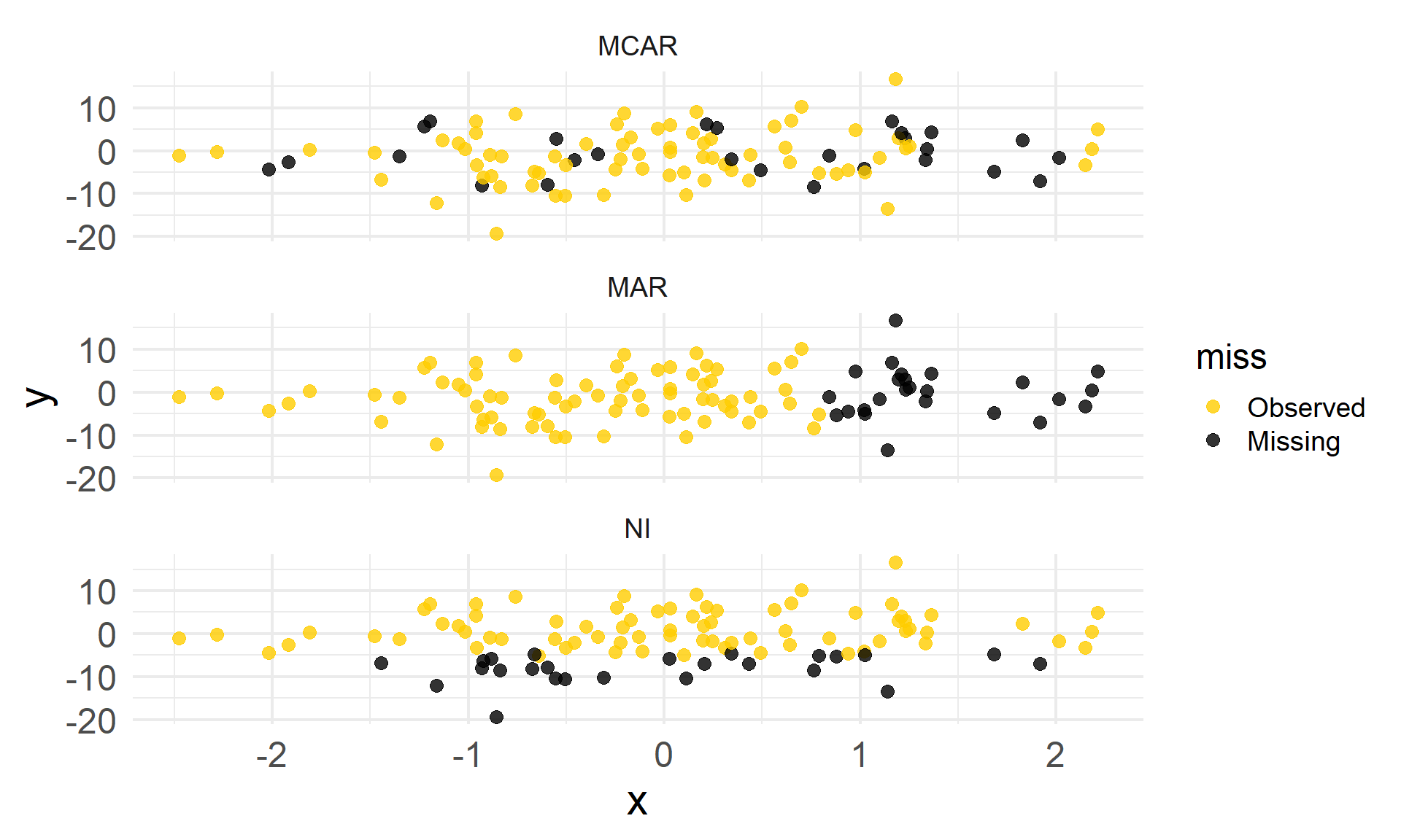
Illustrate with fake data

• N: 100
• X, Z ~ Φ(0, 1), Y = 0.5X - 6Z + ε (let’s pretend Z is unobservable)
• Missingness:
  • MCAR: Complete randomly
  • MAR: Missing Y on the 3rd quantile of X
  • NI: Missing Y on the 3rd quantile of Z

1.3 How do they look like in data

1.4 NI

1.5 Consequence of Missingness

\[Y = \hat \beta_0 + \hat \beta_1 X + \hat \epsilon_i\]

	Summary Stats	Regression	SE vs. complete
MCAR	Unbiased	Unbiased/consistent	Inefficient
MAR	Biased	Unbiased/consistent	Inefficient
NI	Biased	Biased	–

Unbiasedness in MAR is because the censoring of the data is based on an irrelevant variable;

Biasedness in NI is because of the censor with an X within the model

1.6 Dealing with Missing

Ignore it: Listwise deletion (Problem?)

Even for MAR, dropping the entire entry due to the missing would cause bias, because there is no missing in Y but Y is dropped because of the missing of X; cov(X, u) ≠ 0, so often pairwise deletion

Fill it manually: hot deck method (Problem?)

Using neayby approximate values, e.g., mean, the right last-observed observation, The term “hot deck” dates back to the storage of data on punched cards, and indicates that the information donors come from the same dataset as the recipients. The stack of cards was “hot” because it was currently being processed.

Imputation

1. Interpolation
2. Extrapolation
3. Regression imputation: \(M = \boldsymbol{X\gamma} + u\)
   • For multidimentional variable use joint distribution and iterative chain.

(Problems?)

1.7 Better solutions

• Nonparametric modeling: e.g., MICE, KNN Imputation, Missingness Pattern Alternating Lasso, Miss Forest
• Multiple Imputations (MI)
  1. Take multiple guess given estimated distribution (Expectation-Maximization)
  2. Result \(\hat\beta(1), \hat\beta(2), \hat\beta(3)\),… and their variance.
  3. Combine: Rubin’s formula¹

\[\begin{align} \hat\beta =& \frac{\sum^m_{i = 1}\hat\beta_i}{m},\\ var(\hat\beta) =& \frac{\sum^m_{i = 1}var(\hat\beta_i)}{m} + \frac{m + 1}{m}W. \end{align}\]

\(\frac{\sum^m_{i = 1}var(\hat\beta_i)}{m}\) variance within each complete dataset;

\(\frac{m + 1}{m}W\) variance across datasets.

1. \(W = \frac{1}{m}\sum^m var(\hat\beta_i - \bar{\hat\beta})^2\).

1.8 MI

Advantages

Imputations are separated from the analysis ⇒

Misspecification of the model does not affect MI.

Concern

1. Not exactly replicable
2. Rubin’s formula does not always work
   • Esp. for complex models.
3. Time consuming and times to impute.
   • Rule of thumb: 10 (err…)

1.9 When MI Isn’t a Good Idea

1. Model is conditional on X + correctly specified: Listwise would not affect the analysis.
2. Large data: Listwise is trivial.
3. Missingness in X is not a function of Y, and there is no unobserved omitted values that affects Y.
4. There is NI missingness in X: EMs incorrect
5. The model is nonlinear and complicated.
6. Extreme distributional divergence in missing data from multivariate normal.

5% is the rule of thumb, Jakobsen, Janus Christian, Christian Gluud, Jørn Wetterslev, and Per Winkel. 2017. “When and How Should Multiple Imputation Be Used for Handling Missing Data in Randomised Clinical Trials—A Practical Guide with Flowcharts.” BMC Medical Research Methodology 17(1): 162.

What you may try:

Likelihood approach: Estimate distribution and integrate over it (the results are identical no matter how many times doing it), e.g., SEM.

1.10 Some more words about NI

When we know what happened:

Censored data:

Have some information about values of missing data, e.g., all data <0 are coded as 0.

• Leading to heteroscedasticity and nonnormal error
• Solution: For Y missing, two-stage process, 2SLS (Heckman model).

2SLS: Two-Stage least squares

Truncated data:

Have no information about values of missing data, e.g., the data are only observable when it < 100,000

• tobit, use the right distribution—a combination of P(Y_i^* < 0|X) and f(Y_i|X_i).

2 GLM

2.1 Terminology

• Generalized linear regression ≠ general linear regression
• When the very first assumption (“linearity”) of OLS is violated.
  • Most common situation: Noncontinuous Y
• What happened if just using OLS
  1. Unrealistic and nonsensitive predicted outcomes
  2. Heteroscedasticity

But OLS is so beautiful, efficient, and easy!

Solution:

General linear regression is multivariate regression

2.2 Approach: Linear Probability Model (LPM)

\[\begin{align} \pi_i\equiv P(Y = 1|X) =& \beta_0 + \beta_1X_i\\ var(\pi_i) =& \pi(1 - \pi) \\ =& (\beta_0 + \beta_1X_i)[1 - (\beta_0 + \beta_1X_i)] \end{align}\]

The specification of var addresses heteroscedasticity

Pros

Interpreted as OLS + % changes in a unit of X

Cons

Not very reliable transformation

Rule of thumb: 0.2~0.8

1. When X has different ranges, the slope may be not reliable (http://teaching.sociology.ul.ie/bhalpin/wordpress/?p=483; http://teaching.sociology.ul.ie/bhalpin/wordpress/?p=432),

2. unless restrictions are placed on {}, the estimated coefficients can imply probabilities outside the unit interval {}[0,1].

2.3 Approach: Link Function Method

\[P(Y = 1|X) = G(\beta_0 + \beta_1X_1 + ... + \beta_kX_k).\]

• This G() is the link function.
  • When G() = Λ(X), logit (logistic unit)
  • When G() = Φ(X), probit (probability unit)

Logit

The outcome of a binary variable Y_i depends on an unobserved continuous probability Y^*:

\[\begin{align} Y_i =& \begin{cases} 0, \text{if } Y^*\leq 0,\\ 1, \text{if } Y^*> 0.\end{cases}\\ Y^* =& X\beta + u, u\sim \Lambda(0, \frac{\pi^2}{3}) \end{align}\]

Given the PDF of a logistic distribution is \(\Lambda(x) = \frac{e^x}{1 + e^x}\),

\[\begin{align} P(Y_i = 1|X) =& P(Y^* > 0|X) = P(X\beta + u\geq 0|X)\\ =& P(u\geq 0 - X\beta|X)\\ =& 1 - P(u\leq - X\beta|X) = 1 - \Lambda(-X\beta)\\ =& 1 - \frac{e^{-X\beta}}{1 + e^{-X\beta}}\\ =& \frac{1}{1 + e^{-X\beta}} = \frac{e^{XP}}{1 + e^{X\beta}} = \Lambda(X\beta)\\ P(Y_i = 0|X) =& P(X\beta + u \leq 0 |X) = P(u \leq -X\beta |X)\\ =& \Lambda(-X\beta) = \frac{e^{-X\beta}}{1 + e^{-X\beta}} = \frac{1}{1 + e^{X\beta}}\\ =& 1 - \Lambda(X\beta) \end{align}\]

Probit

\[\begin{align} Y_i =& \begin{cases} 0, \text{if } Y^*\leq 0,\\ 1, \text{if } Y^*> 0.\end{cases}\\ Y^* =& X\beta + u, u\sim \Phi(0, 1)\\ \text{Similarly, } P(Y_i = 1|X) =& 1 - \Phi(-X\beta)\\ f(x) =&\frac{1}{\sqrt{2\pi}\sigma}e^{-\frac{(x - \mu)^2}{2\sigma^2}} \end{align}\]

2.4 Logit vs. Probit

• Probit is a little more computationally costly than logit ( \(\frac{e^x}{1 + e^x}\) vs. \(\frac{1}{\sqrt{2\pi}\sigma}e^{-\frac{(x - \mu)^2}{2\sigma^2}}\))

• Logit and probit coefficients are identical but on different scales (var_logit = π²/3, var_probit = 1)

Let’s say the true model is a logit, but we estimate a probit model

\[\begin{align} P(Y = 1|X) =& 1 - P(u \leq -X\beta_{probit}|X)\\ =& 1 - \Phi(\frac{-X\beta_{probit}}{\pi^2/3})\\ =& 1 - \Lambda(-X\beta_{logit})\\ \Leftrightarrow\ \beta_{logit} =& \frac{\sqrt{3}}{\pi}\beta_{probit}\approx 0.55\beta_{probit} \end{align}\]

2.5 Estimation

Minimize the least square? No~

The maximum likelihood estimation:

\[\mathcal{L}(\hat\theta|Y, X, m) \equiv \mathcal{L}(\hat\theta|Y, X) = k(Y)f(Y|\hat\theta, X)\propto f(Y|\hat\theta, X)\]

Define: \(\hat\theta = argmax_{\theta^*}\mathcal{L}(Y|X, \theta^*)\), the .red[maximum likelihood estimate] of θ from among all possible values of θ^*

We cannot minimize the least square as in OLS, since Y^* is not observed (unable to calculate \((Y - \bar Y)^2\) ). So, one has to use the likelihood approach to inferenceb i.e., the maximum likelihood estimation:

m: a model

θ: parameter

k: an arbitrary function, depending on the data.

argmax: when having the argument, the function get the max

\[\begin{align} \mathcal{L}(\beta|Y, X) =& \Pi_{y = 1}P(Y = 1|X)\Pi_{y = 0}P(Y = 0|X)\\ =& \Pi_{y = 1}F(X\beta)\Pi_{y = 0}[1 - F(X\beta)]\\ \Leftrightarrow\ ln(\mathcal{L}) =& \sum ln[F(X\beta)] + \sum ln[1 - F(X\beta)] \end{align}\]

• If there is an analytic solution, calculate it.
• If no, computational approaches, e.g., Hill-climber (small step iteration) and Newton-Raphson (large step after detecting a deep slop, i.e., a fast acceleration).

Property:

1. Consistent;
2. Asymptotically unbiased;
3. Generally asymptotically efficient.

Asymptotical: 渐进式的

2.6 Interpretation

\[P(Y = 1|X) = \frac{e^{XP}}{1 + e^{X\beta}}\]

What’s the effect of every one unit change of X on P(Y = 1|X)?

Ways to interpret GLM outcomes:

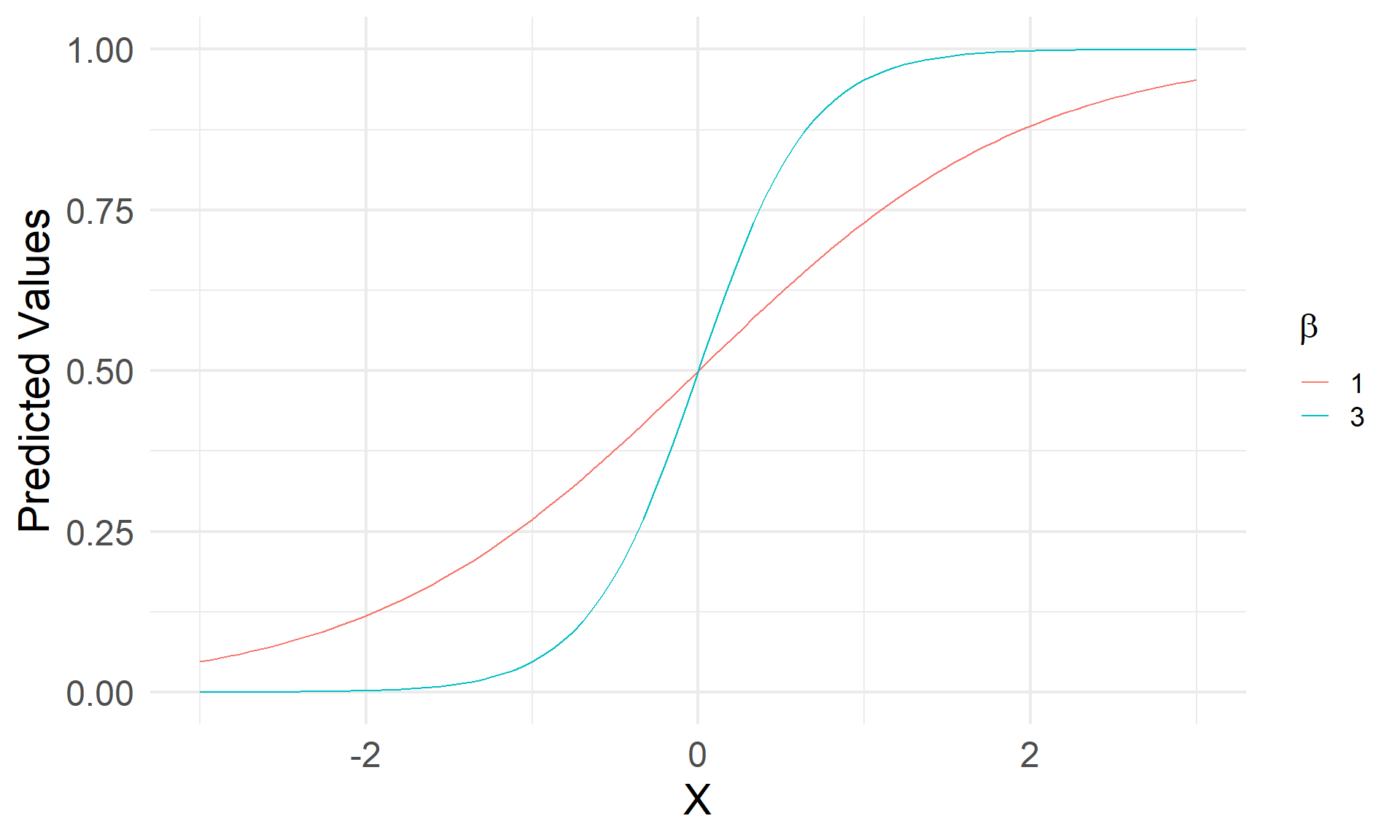
1. Predicted value plots
2. Marginal effect
3. First difference

2.7 Predicted Value Plots

Compare when beta equals different values, the larger the more s

2.8 Goodness of Fit

Psedo-R²

Several ways to estimate it, but none of them is quite straightforward.

Proportional reduction in error (PRE), a.k.a., Percent correctly predicted (PCP)

Comparing estimates of P(Y = 1|X) to Y: If P(Y = 1|X) > 0.5, define Ŷ = 1, otherwise, Ŷ = 0. Let’s denote

	Y = 1	Y = 0
Ŷ = 1	n11	n01
Ŷ = 0	n10	n00

\[PCP = \frac{n_{11} + n_{00}}{\sum n}\]

Advanced: How much better the model predict than plain guess. Define PMC as the percent modal category (the plain guess). That is,

\[PRE = \frac{PCP - PMC}{1 - PMC}\]

An advanced version is ePRE.

ePRE: expected PRE, Herron 1999, PA

2.9 Take-home point

2.10 The Journey

Appendix

2.11 Marginal Effects of GLM

The instantaneous change

\[\begin{align} &\frac{\partial P(Y = 1|X)}{\partial X} \\ =& \beta_1e^{\beta_0 + \beta_1X_1 + \beta_2X_2}(1 + e^{\beta_0 + \beta_1X_1 + \beta_2X_2})^{-1}\\ & -e^{\beta_0 + \beta_1X_1 + \beta_2X_2}(1 + e^{\beta_0 + \beta_1X_1 + \beta_2X_2})^2\beta_1e^{\beta_0 + \beta_1X_1 + \beta_2X_2}\\ =& \frac{\beta_1e^{\beta_0 + \beta_1X_1 + \beta_2X_2}(1 + e^{\beta_0 + \beta_1X_1 + \beta_2X_2}) - e^{\beta_0 + \beta_1X_1 + \beta_2X_2}\beta_1e^{\beta_0 + \beta_1X_1 + \beta_2X_2}}{(1 + e^{\beta_0 + \beta_1X_1 + \beta_2X_2})^2}\\ =& \frac{\beta_1e^{\beta_0 + \beta_1X_1 + \beta_2X_2}}{(1 + e^{\beta_0 + \beta_1X_1 + \beta_2X_2})^2} = \beta_1(\frac{e^{\beta_0 + \beta_1X_1 + \beta_2X_2}}{1 + e^{\beta_0 + \beta_1X_1 + \beta_2X_2}})(\frac{1}{1 + e^{\beta_0 + \beta_1X_1 + \beta_2X_2}}) \\ =& \beta_1P(Y = 1|X)P(Y = 0|X) \end{align}\]

The margin has the maximum value when P(Y = 1|X) = P(Y = 0|X) = 0.5, or saying Xβ = 0. In other words, marginal effect depends on the value of X.

In fact, it depends on the value of .red[all the X]. This requires the report of marginal effect including the value of the Xs.

2.12 First Difference

The discrete version of marginal effect.¹

\[FD: P(Y|X = X_k^H, X_{-k}) - P(Y|X = X_k^L, X_{-k})\]

X_k^H,L:

1. Max → Min
2. Median/mean ± σ_Xk
3. Two theoretical interesting values
4. Discrete: 0/1
5. Compound change: Change more than one variable once, since some of them often change together, e.g., eco level and edu level.

1. X_-k: All other independent variables (holding them constant); Usually mean or median. The median is sometimes nicer because it can fit both ordinal and continuous variables.

2.13 Uncertainty of Marginal Effects and FDs

1. Mathematical: Approximating with the delta method.
2. Simulation: It is nice since one variable may not (often not) have symmetric distributions.
3. Just using the variance of \(X\hat\beta\).

Stretch

https://www.bilibili.com/video/BV1E54y1r76o/?buvid=Y045340D2FD9FA3A46419EEFE4578279ECBD&from_spmid=main.space-search.0.0&is_story_h5=false&mid=7RnjBONLRMus4FQZFBWD2g%3D%3D&p=2&plat_id=114&share_from=ugc&share_medium=iphone&share_plat=ios&share_session_id=79FE08C9-F2B1-4C18-A16C-B31179817B42&share_source=WEIXIN&share_tag=s_i&timestamp=1728732278&unique_k=skSWw7j&up_id=390316092&vd_source=f38aeefd0d38cecba9017eeee43e71c8

Meditation

松茸的世界：5分钟正念冥想-自信之心

https://www.xiaoyuzhoufm.com/episode/65b752ed0bef6c207457f51b?s=eyJ1IjogIjYwNDA1OGJiZTBmNWU3MjNiYmY3MjZiZSJ9