Model Specification

Large N & Leeuwenhoek (70700173)

Yue Hu

Overview

1. Nonstochastic X (“X is fixed”), and X has positive noninfinite variance (σ_X > 0);
2. Correct specification;
3. Linearity in the parameter;
4. Full rank/identification
   • N > K; K = 2 for a simple OLS);
5. Mean zero errors
   • E(ε_i|X_i) = 0;
6. Exogeneity: No covariance between X_i and ε_i
   • E(X_iε_i) = cov(x_i, ε_i) =0;

7. No autocorrelation/serial correlation: E(ε_i, ε_J|X_i, X_j) = cov(ε_i, ε_J|X_i, X_j) = 0, ∀ i, j);
8. Normality: \(U|X \sim N(0, \sigma^2I).\)
9. Homoskedasticity/Spherical disturbances: constant variance of ε_i, var(ε_i|X) = σ²;
10. No perfect collinearity: there are more than one X, ∄ X_i s.t., X_i = a + b∑_{j = 1}b_jX_j

Specification Issues

How can you specify things wrong?

Measurement Issues

• Proxy variable
• Measurement error
• Variable type

Specification Issues

• Functional form
• Omitted variable

Interpretation Issues

• Nonlinear model

1 Measurement Issues

1.1 Why proxy variables?

• Human capital ← years of education
• GDP ← economic well-being
• Voter turnout ← democratic health
• Partisaship ← ideology

1.2 Proxy Variable in Statistics

True model: Y = β₀ + β₁X₁ + β₂X₂ + β₃X₃^* + ε, ε ~ Φ(0, σ_ε²).

• Unobservable: X₃^*.
  • Observable X₃^* = δ₀ + δ₁X₃ + ν, ν ~ Φ(0, σ_ν²).
• ⇒ Y = (β₀ + β₃δ₀) + β₁X₁ + β₂X₂ + β₃δ₁X₃ + (ε + β₃ν).
  • Assuming cov(ε, ν) = 0, then
    1. E(ε + β₃ν|X) = 0;
    2. var(ε + β₃ν|X) = β₃²σ_ν² + σ_ε².

cov(u,v) = 0: u, v independent

Outcome of proxy variable

Only when cov(ε, X₃) = cov(ν, X₁) = cov(ν, X₂) = 0, can the model produce unbiased estimates.

1.3 Measurement Error

Relation with proxy variable

Proxy variable is a source of measurement error (random error, specifically).

• Nonrandom error → systematic bias
• Random error in the outcome variable: Y = Y^* + ε.
  • \[\begin{align} &Y^* = \beta_0 + \beta_1X_1 +\cdots+ \beta_kX_k + \epsilon;\\ &Y = \beta_0 + \beta_1X_1 +\cdots+ \beta_kX_k + (\nu + \epsilon) \end{align}\]
  • Consequence
    • β Unbiased
    • var(β) ↑

1.4 Measurement Error

• Random error in the explanatory: X = X^* + ν. If E(νX) = 0, then \[\begin{align} Y =& \beta_0 + \beta_1(X_1 - \nu) + \epsilon,\\ =& \beta_0 + \beta_1X_1 + (\epsilon - \beta_1\nu). \end{align}\]

\[\begin{align} cov(\epsilon, X_1) =& E(\epsilon X_1) - E(\epsilon)E(X_1) = E(\epsilon X_1), \\ =& E[\epsilon (X_1^* + v)] = E(\epsilon X_1^*) + E(\epsilon v) = \sigma_\epsilon^2\neq0.\\ cov(\epsilon - \beta_1\nu, X_1) =& cov(-\beta_1\nu, X_1) = -\beta_1cov(\nu, X_1) = -\beta_1\sigma_\nu^2.\\ \Rightarrow\ plim(\hat\beta_1) =& \beta_1 + \frac{cov(\epsilon - \beta_1\nu, X_1)}{var(X_1)},\\ =& \beta_1 + \frac{-\beta_1\sigma_\nu^2}{\sigma_{X_1}^2} = \beta_1 + \frac{-\beta_1\sigma_\nu^2}{\sigma_{X_1}^{*2} + \sigma^2_\epsilon} = \frac{\sigma_{X_1}^{*2}}{\sigma_{X_1}^{*2} + \sigma^2_\nu}\beta_1. \end{align}\]

plim: probability limit operation, convergence in probability

1.5 Measurement Error

\[plim(\hat\beta_1) = \frac{\sigma_{X_1}^{*2}}{\sigma_{X_1}^{*2} + \sigma^2_\nu}\beta_1.\]

• Unbiased only when var(X₁) = var(X₁^* + ν), i.e., σ²_X1 = σX₁^*2+ σ_ν²
• Consequence: \(|\hat\beta_1| < \beta_1\), a.k.a., the attenuation bias.
  • β₁: underestimated;
  • Affecting the estimations of others in unknown ways .

1.6 Bonus: Concerns of the variable type

Warning

In OLS, there is no requirement (assumption) for Xs (but the parameter) to be linear.

• Indicator variable (binary)
  • \(Y = \beta_0 + \beta_1X_i + \epsilon_i,\) where X is either male (0) or female(1)
    • β₀: E(Y|X = male);
    • β₁: E(Y|X = female) - E(Y|X = male).
• Nominal:
  • Can’t regress unless being broken up into indicators
  • e.g., A race variable: white, black, native
    • H₀: β_black = 0, testing the difference between black and white
    • H₀: β_black = β_native = 0, testing if the race has any effect.

In a regression, the information of the baseline is captured by the intercept

1.7 If no linearity requirement for Xs, why transformation

You saw log(GDP) or log(income), right? What does the logarithm transformation do?

Some may say making X more linear? However, no assumption on X

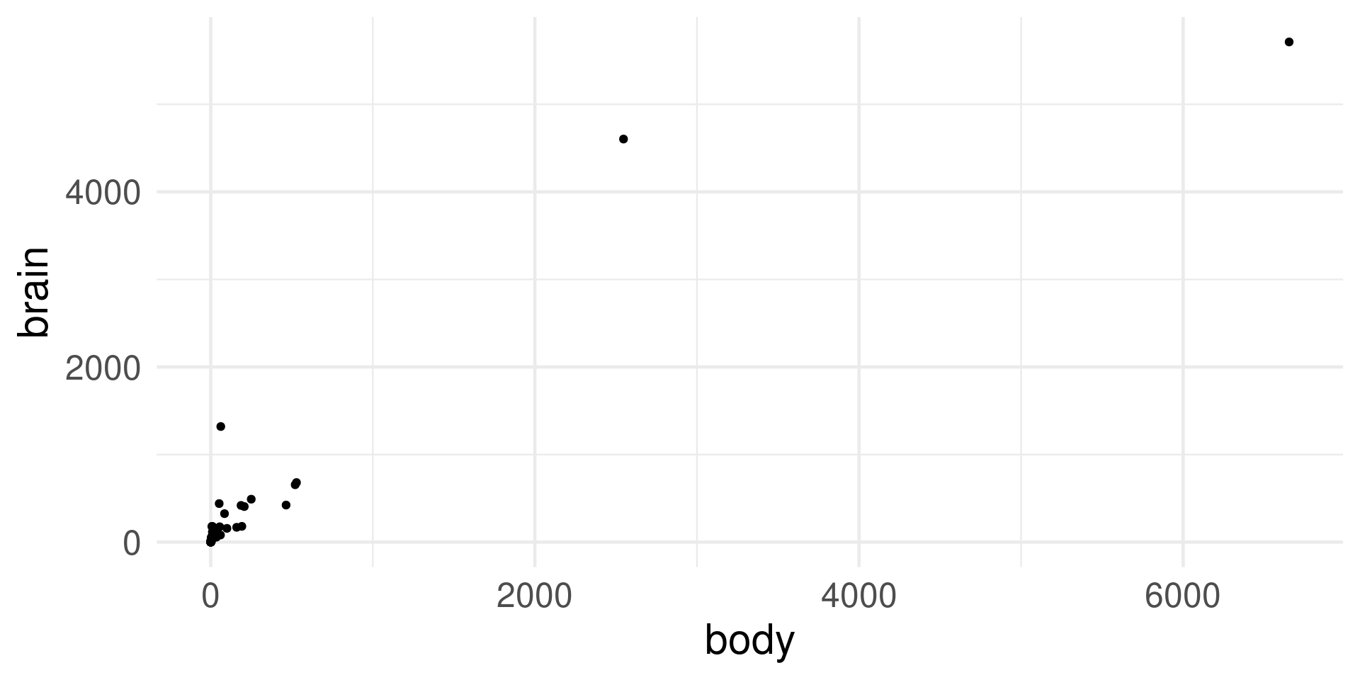
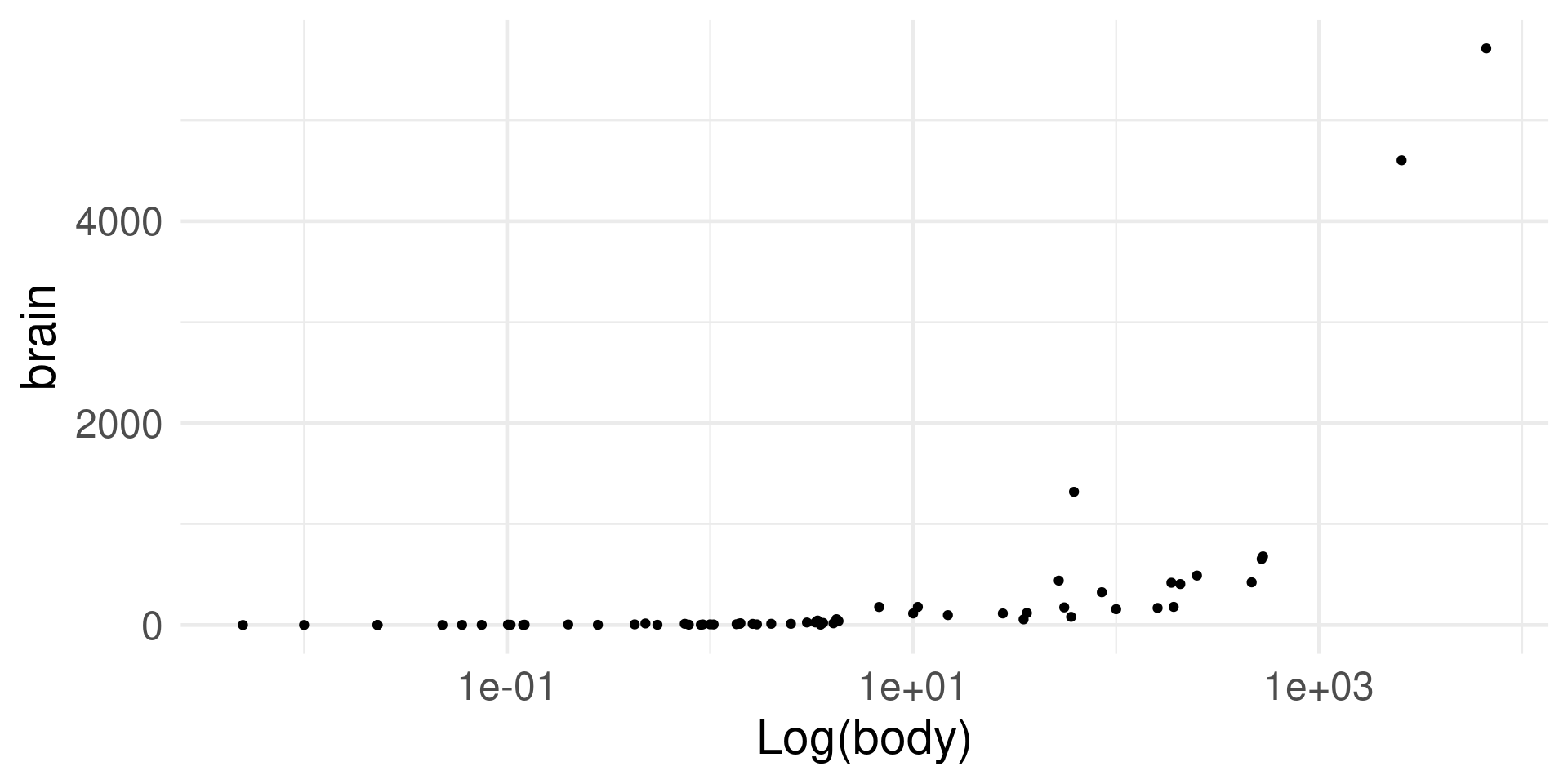
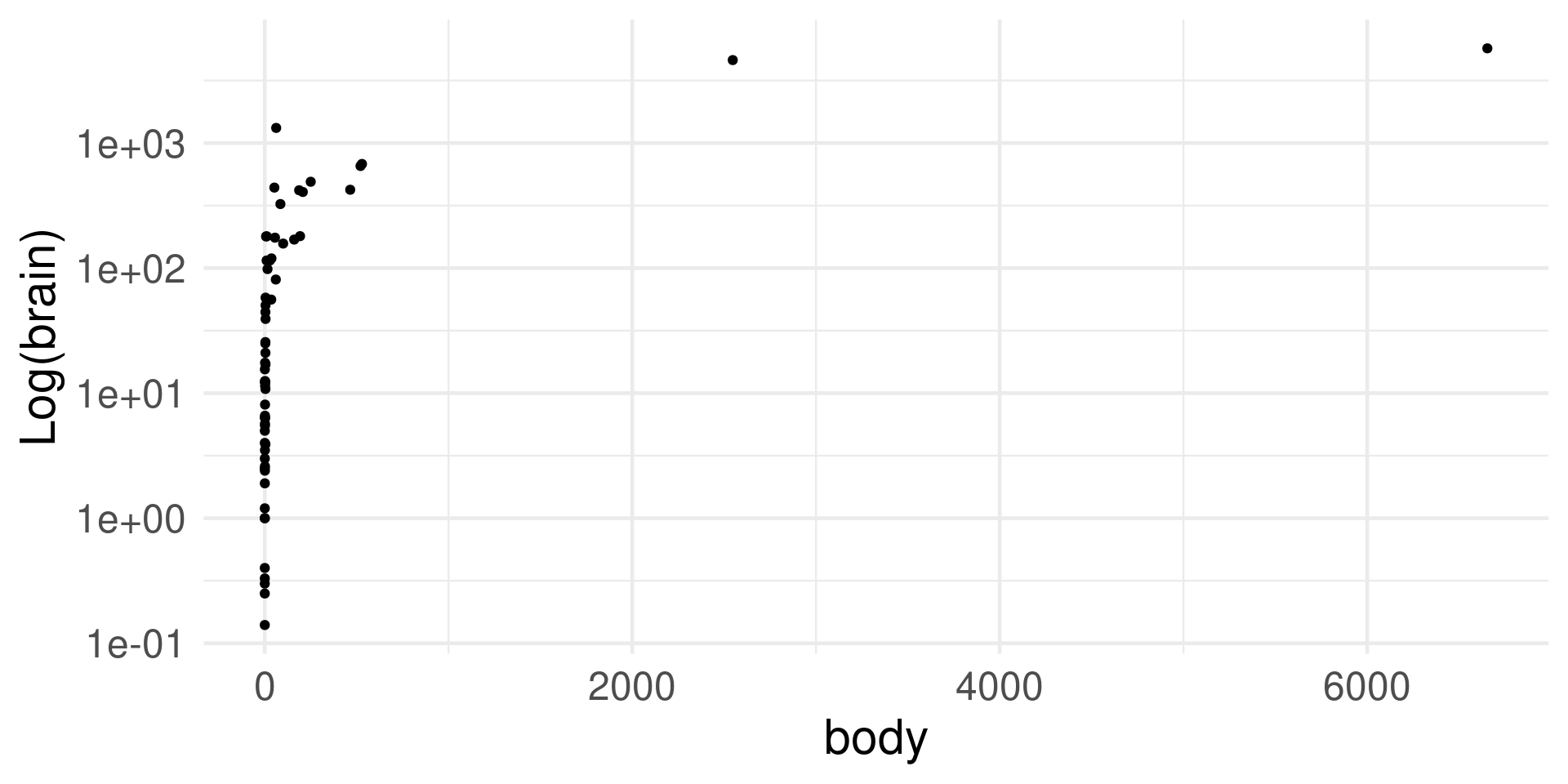
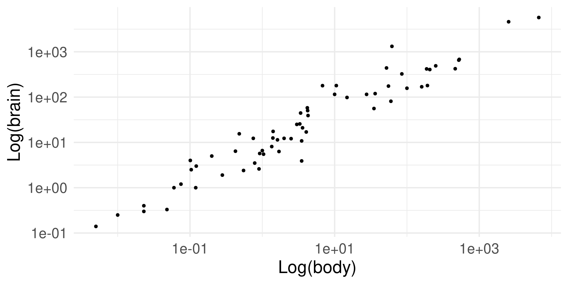
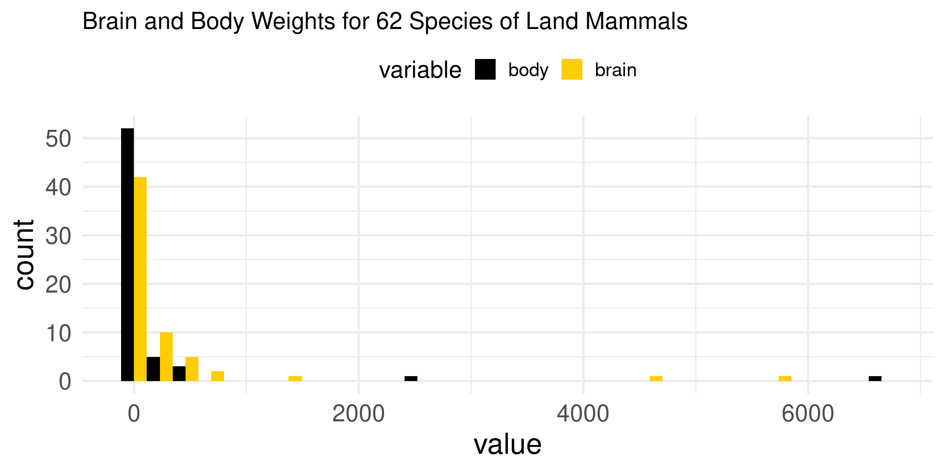
The problem to solve: Violation of A3 (“Linearity in the parameter”)

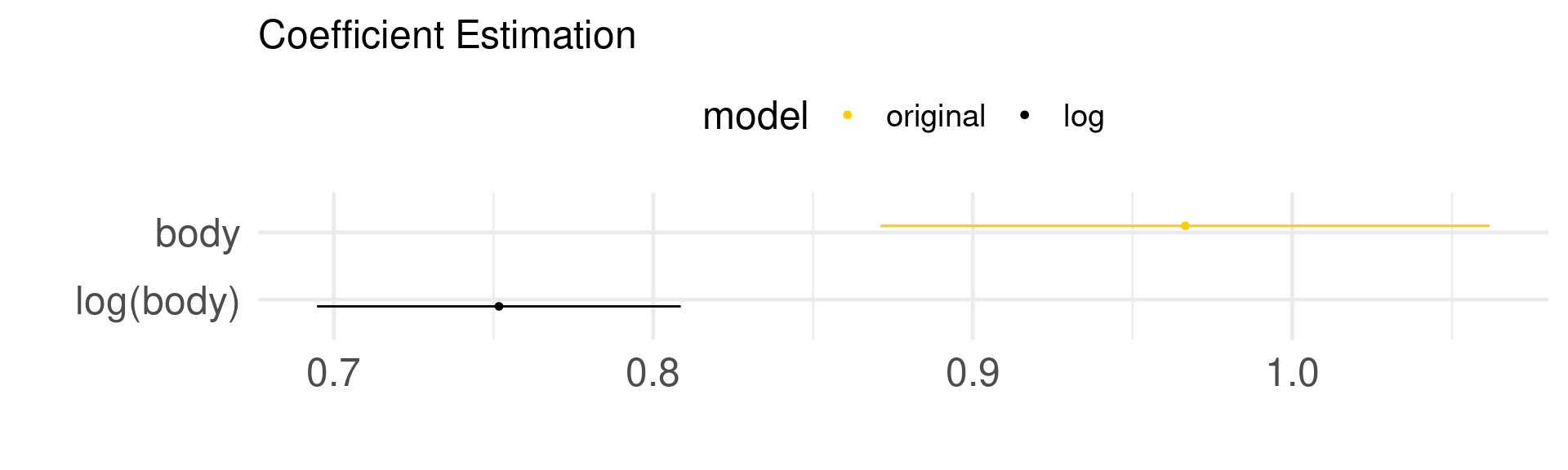
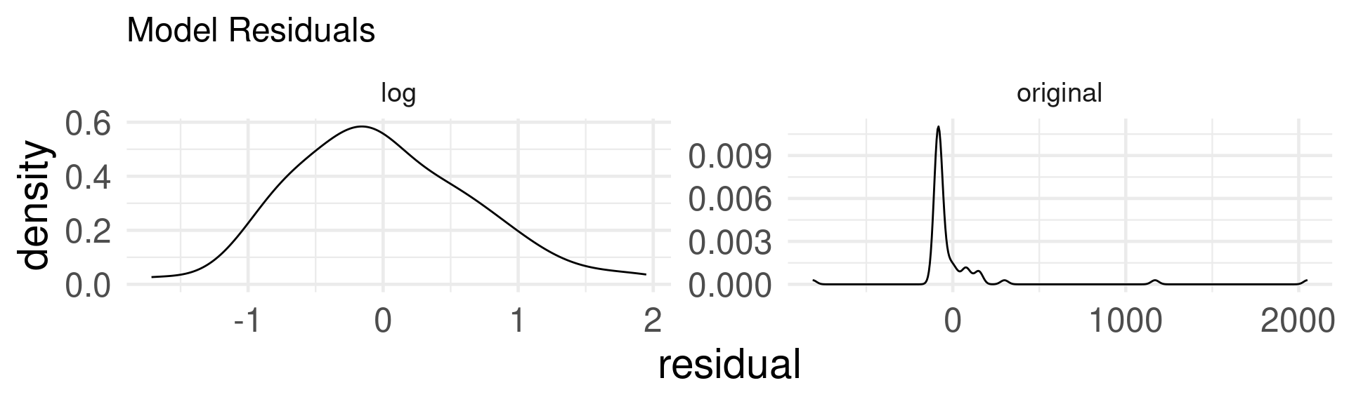
1.8 Model Fit with Logarithm Transformation

1.9 So, when to use Logrithm Transformation

Critical criterion: Skewness

Rule of thumb:

• |Skewness| < 0.5, the distribution is approximately symmetric (0 ⇔ perfect symmetric)
• |Skewness| < 1, moderately skewed
• |Skewness| > 1, highly skewed

Example data:

$body
[1] 6.249429

$brain
[1] 4.828829

2 Misspecification

2.1 Problem Types

1. Functional form
2. Omitted variable

2.2 Misspecification in the Functional Form

When there are two ways to specify the model:

\[\begin{align} Y =& f_1(X_1, X_2, X_3) =\beta_1X_1 + \beta_2X_2 + \beta_3X_3 + \epsilon, \\ Y =& f_2(X_1, X_2, X_3) =\beta_4X_1^2 + \beta_5X_2^3 + \beta_6X_3^4 + \epsilon. \end{align}\]

Which specification is correct?

Test out:

β₁ in Y = f₁(X) + f₂(X) + ε

Conduct a joint test:

H₀: β₁ = β₂ = β₃ = 0 or

β₄ = β₅ = β₆ = 0

Only one true model!

Let’s assume f₁ is the true model:

\[var(\hat\beta_1) = \frac{\sigma^2}{(X_1 - \bar X_1)^2(1 - \rho_{12})}.\]

ρ₁₂: Correlations between X₁ and X₂, such as between X and X². So, when ρ₁₂ ↑ variance is inflated when ρ₁₂ ↑

Statistics: Davidson-Mackinnon test

1. Run \(Y = f_2(X) + \epsilon\) and calculate the expected value \(\hat Y = E[Y|f_2(X)]\)
2. Run \(Y = f_1(X) + \theta\hat Y + \epsilon\), and test if θ = 0.

2.3 Omitted Variable

\[\begin{align} True: Y_i =& \beta_0 + \beta_1X_{1i} + \beta_2X_{2i} + \epsilon_i;\\ Specified: Y_i =& \tilde\beta_0 + \tilde\beta_1X_{1i} + \tilde \epsilon_i, \end{align}\]

How does \(\tilde\beta_1\) compare to \(\beta_1\)?

\[\begin{align} Y_i =& \beta_0 + \beta_1X_{1} + \beta_2X_{2} + \epsilon_i,\\ Y_i -\bar Y =& \beta_1(X_{1} - \bar X_1) + \beta_2(X_{2} - \bar X_2) + (\epsilon_i - \bar \epsilon),\\ (Y_i -\bar Y)(X_1 - \bar X_1) =& \beta_1(X_{1} - \bar X_1)^2 + \beta_2(X_{2} - \bar X_2)(X_1 - \bar X_1)\\ &+ (\epsilon_i - \bar \epsilon)(X_1 - \bar X_1),\\ \frac{(Y_i -\bar Y)(X_1 - \bar X_1)}{\sum(X_1 - \bar X_1)^2} =& \beta_1\frac{\sum(X_{1} - \bar X_1)^2}{\sum(X_1 - \bar X_1)^2} + \beta_2\frac{\sum(X_{2} - \bar X_2)(X_1 - \bar X_1)}{\sum(X_1 - \bar X_1)^2} + \frac{\sum \epsilon_i(X_1 - \bar X_1)}{\sum(X_1 - \bar X_1)^2}.\\ \text{That is, } \tilde\beta_1 =& \beta_1 + \beta_2\hat\delta_1 + \frac{\sum \epsilon_i(X_1 - \bar X_1)}{\sum(X_1 - \bar X_1)^2},\\ \Rightarrow E(\tilde\beta_1|X_1) =& E(\beta_1|X_1) + E(\beta_2\hat\delta_1|X_1) + E[\frac{\sum \epsilon_i(X_1 - \bar X_1)}{\sum(X_1 - \bar X_1)^2}|X_1],\\ =& \hat\beta_1 + \hat\beta_2E(\hat\delta_1|X_1) + \frac{\sum(X_1 - \bar X_1)}{\sum(X_1 - \bar X_1)^2}E(\epsilon_i|X_1),\\ =& \hat\beta_1 + \hat\beta_2\delta_1. \end{align}\]

2.4 Biased how

\[E(\tilde\beta_1|X_1) = \hat\beta_1 + \hat\beta_2\delta_1,\] in which \(\hat\delta_1\) is the regression coefficient of \(X_2\) on \(X_1\) ( \(X_1 = \delta_0 + \delta_1X_2 + r\)).

• \(\tilde\beta_1\): Biased, unless X₂ is an irrelevant variable.
  • Even if δ₁ = 0, \(X_1 = \delta_0 + r\), the model may increase the risk of Type I error

False positive

How About the Residual?

\[Y_i = \beta_0 + \beta_1X_{1} + \epsilon,\]

\[\epsilon = \beta_2X_{2} + \epsilon_i.\]

\(E(\epsilon|X_1) = E(\beta_2X_{2} + \epsilon_i) = \beta\mu_2\neq0\)

• Against the assumption.

\(var(\epsilon|X_1) = var(\beta_2X_{2} + \epsilon_i|X_1)= \beta_2^2\sigma_2^2 + \sigma_u^2 + 2\beta_2cov(X2, u) = \beta_2^2\sigma_2^2 + \sigma_u^2\)

• All values are fixed, that is, still homoscedasitic.

\(E(X_1\epsilon) = \beta_2[cov(X_1,X_2) - \mu_{X_1}\mu_{X_2}],\)

• When cov(X₁, X₂)≠0 ⇒ Increase the difficulty to isolate X from u.

\(E(\epsilon_i\epsilon_j|X_i)\neq 0\)

\[\begin{align} E(\epsilon_i\epsilon_j) - E(\epsilon_i)E(\epsilon_j) =& E[(\beta_2X_{2i} + \epsilon_i)(\beta_2X_{2j} + \epsilon_j)] - \beta_2^2\mu^2_{X_2},\\ =& E(\beta_2^2X_{2i}X_{2j} + \beta_2^2X_{2i}u_{j} + \beta_2^2X_{2j}u_{i} + \epsilon_i\epsilon_j) - \beta_2^2\mu^2_{X_2},\\ =& \beta_2^2E(X_{2i}X_{2j}) - \beta_2^2\mu^2_{X_2},\\ =& \beta_2^2cov(X_{2i}, X_{2j}) - \beta_2^2\mu^2_{X_2} + \beta_2^2\mu^2_{X_2},\\ =& \beta_2^2cov(X_{2i}, X_{2j}). \end{align}\]

\[\begin{align} E(X_1\epsilon) =& E[X_1(\beta_2X_2 + u)], \\ =& E(X_1\beta_2X_2) + E(X_1u),\\ =& \beta_2E(X_1X_2),\\ =& \beta_2[cov(X_1,X_2) - \mu_{X_1}\mu_{X_2}]. \end{align}\]

• When cov(X₁, X₂) ≠ 0, E(X₁ε) ≠ 0.

Examples:

• Economic development and democracy
• Election and democracy
• Media freedom and political accountability

3 Misinterpretation

3.1 Linear modeling of nonlinear relationship

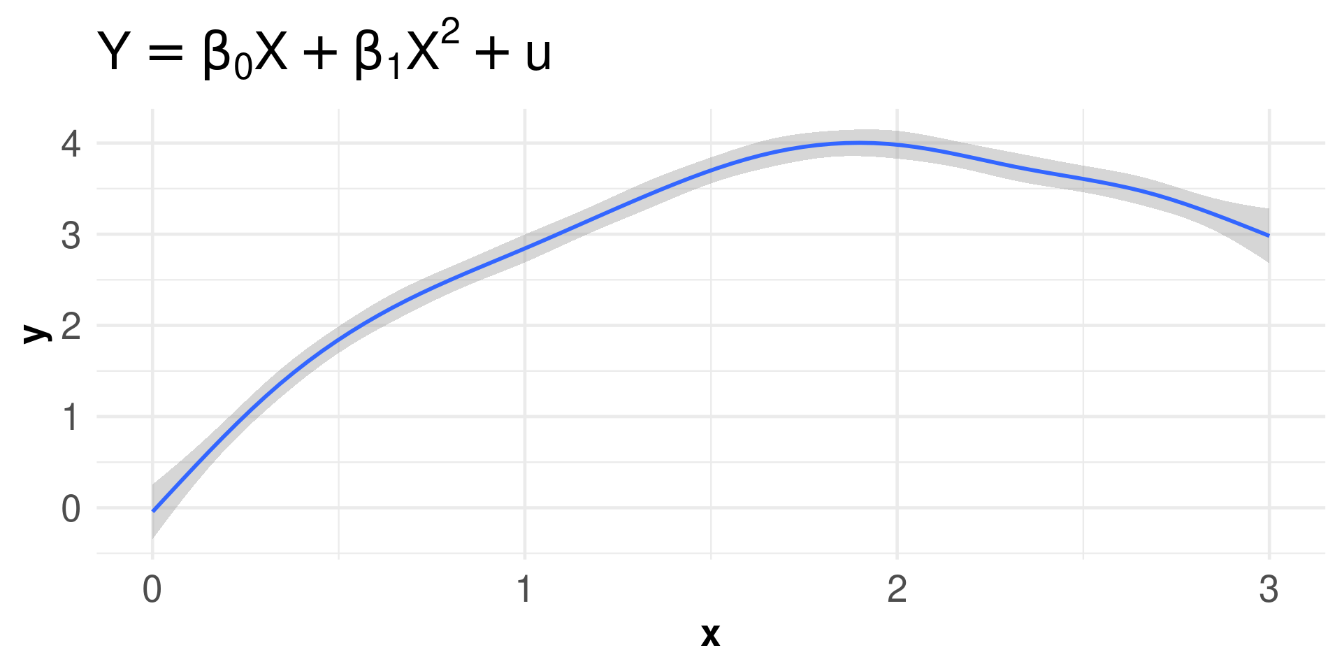
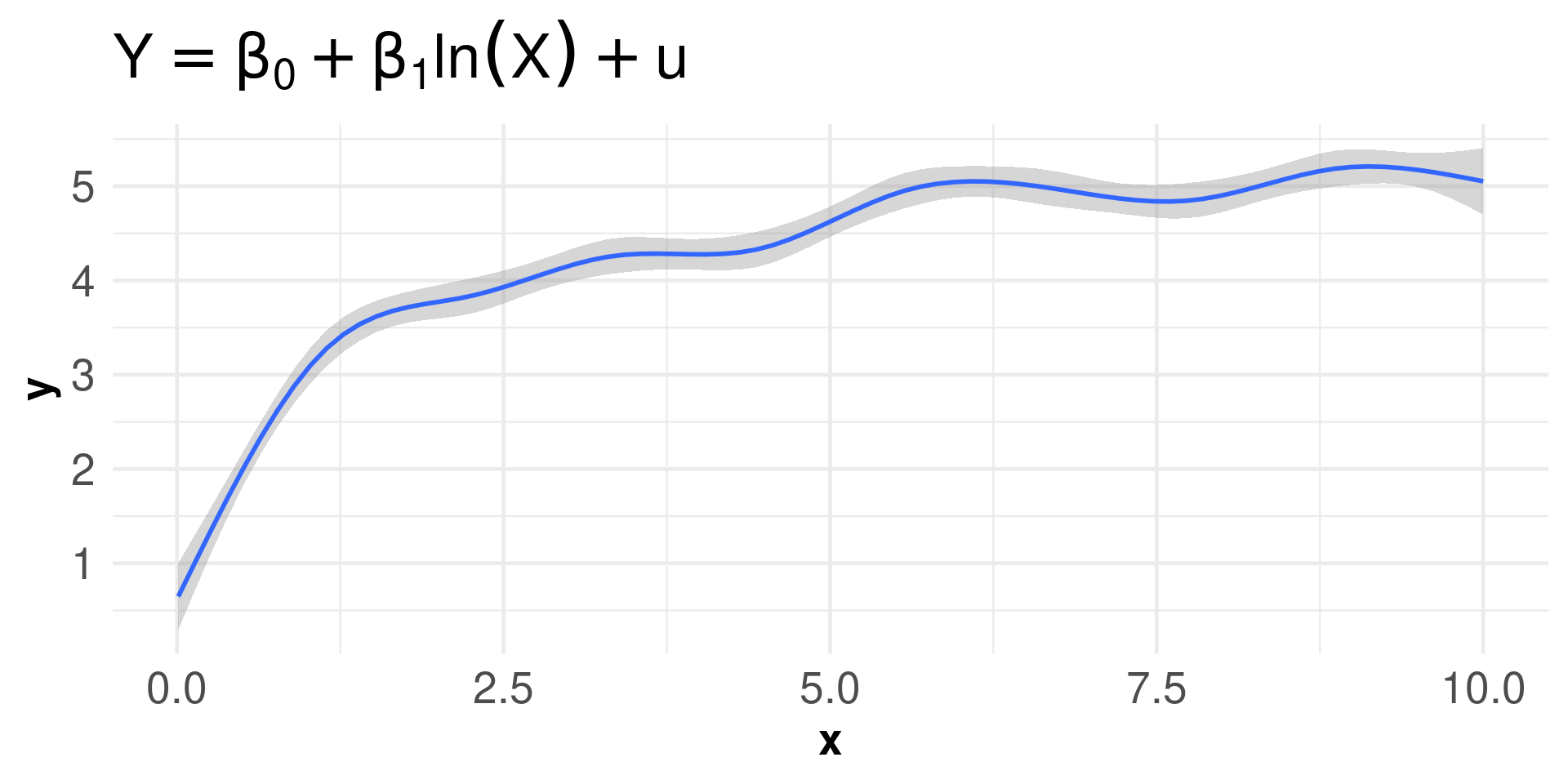
Believe or not, still unbiased & efficient linear estimates, but what does β₁ mean?

Linear combination means adding together

3.2 One way out

Marginal Effects💫

Discrete:

\[Pr(Y|x = X_{n + 1}) - Pr(Y|x = X_n)\]

Continuous:

\[\lim_{\Delta x\to0} \frac{ f(x + \Delta x) - f(x)}{\Delta x}\]

That’s to say, every value in X (n > 1) has a marginal effect (Δ_x). Which one should we use?

3.3 Marginal Effects in Types

Average Marginal Effect (AME)

1. Calculate the marginal effect of each variable x for each observation.
2. Calculate the average.

Marginal Effect at the Mean (MEM)

Calculate the marginal effect of each variable x for each’s mean value.

Marginal Effect at Representative Values (MER) 🌟

Calculate the marginal effect of each variable x for value(s) of interest.

3.4 Hypothesis Testing of A Nonlinear Model

\[e.g., Y = \beta_0 + \beta_1X + \beta_2X^2 + u.\]

• Margins: \(\frac{\partial Y}{\partial X} = \beta_1 + 2\beta_2X\)
• Let α = 0.05, H₀: β₁ + 2β₂X = 0;
  • The average acceleration is zero

Statistics:

\[\begin{align} \frac{\beta_1 + 2\beta_2X - 0}{SE(\beta_1 + 2\beta_2X)}\sim& t_{n - 3}.\\ SE(\beta_1 + 2\beta_2X) =& \sqrt{var(\beta_1 + 2\beta_2X)}, \\ =& \sqrt{var(\beta_1) + 4X^2var(\beta_2) + 4Xcov(\hat\beta_1,\hat\beta_2)}. \end{align}\]

3.5 Interpretation

Statistics:

\[\begin{align} \frac{\beta_1 + 2\beta_2X - 0}{SE(\beta_1 + 2\beta_2X)}\sim& t_{n - 3}.\\ \end{align}\]

Interpretation issue

Can’t simply say whether the null hypothesis is rejected, because there may not be a coherent effect over the entire domain of X due to the nonlinearity.

• Way-out: “In the range from a to b, the hypothesis can be rejected.”
  • Max - min/First difference
  • Marginal effects across values
  • Just plot it. (Do this, cool kids!)

Take-home point

Appendix

Stretch

https://www.bilibili.com/video/BV1E54y1r76o/?buvid=Y045340D2FD9FA3A46419EEFE4578279ECBD&from_spmid=main.space-search.0.0&is_story_h5=false&mid=7RnjBONLRMus4FQZFBWD2g%3D%3D&p=2&plat_id=114&share_from=ugc&share_medium=iphone&share_plat=ios&share_session_id=79FE08C9-F2B1-4C18-A16C-B31179817B42&share_source=WEIXIN&share_tag=s_i&timestamp=1728732278&unique_k=skSWw7j&up_id=390316092&vd_source=f38aeefd0d38cecba9017eeee43e71c8

Meditation

松茸的世界：5分钟正念冥想-自信之心

https://www.xiaoyuzhoufm.com/episode/65b752ed0bef6c207457f51b?s=eyJ1IjogIjYwNDA1OGJiZTBmNWU3MjNiYmY3MjZiZSJ9