社会网络分析: 分析网络

政务大数据应用与分析 (80700673)

胡悦

清华大学社会科学学院

概要

理解网络

目的：描述网络结构，识别网络特征

• 网络方法论 ✓
• 网络要素 ✓
• 自我中心网络 ✓

分析网络

目的：揭示网络构成因素和原因

• 邻居分析（“近景”）
• 扩散分析（“中景”）
• 全网分析（“远景”）*

1 邻居分析

1.1 邻居类型

1. Dyads
2. Triads
3. Communities

1.2 Dyads Distribution

1. None: A   B
2. Arc: A → B; B ← C
3. Reciprocal: A ↔︎ B

Arc is a directed edge

Both are using the described the same phenomenon

• Dyadic: \[R = \frac{\#Reciprocated\ Pairs}{\# Connected\ Pairs}\]

• Arc: \[R = \frac{\#Reciprocated\ Arcs}{\# Total\ Arcs}\]

1.3 Triads

A、B、C三方，存在几种建立关系的方式?

(2²)³ = 64

Triad census, Prell and Skvoretz (2008), fig. 1

1.4 Transitive Triads

A→B→C + A→C

Prell and Skvoretz (2008), fig. 1

1.5 Vacuous Triads

Prell and Skvoretz (2008), fig. 1

/v’ækjuəs/

No feature a directed path

Used to study social capital: closure (all nodes are reciprocal) and brokerage

1.6 Dyads in triads

• Simmelian tie: Dyads 同时与第三方有互惠关系
  • Dyads more stable when embedded in triads

1.7 应用

定义网络结构平衡（Structural Balance）

Maoz et al. (2007)

The enemy of my enemy is my friends.

过往186年中，IR充满了imbalance, 友之敌为友，友by alliances, 敌military disputes

Realistic factors increase imbalance: strategic rivalry, opportunism and exploitative tendencies, capability parity, and contiguity

Liberal factors reduce it: joint democracy, economic interdependence, shared IGO membership

1.8 Community: Beyond k-ads

小世界, Klovdahl et al. (1994)

• 695 人
• 平均距离为大约5步
• 平均每人3步内就能覆盖75个其他人

Disneyland: it’s a small world

超越strong, presented ties，小世界网络是一类特殊的复杂网络结构，在这种网络中大部分的节点彼此并不相连，但绝大部分节点之间经过少数几步就可到达，比如六度空间理论（实际可能在2左右，最长不过8）

Reachability in Colorado Springs

• Epidemic Potential in Human Sexual Networks
• sexual contact only, STD
• High-risk actors over 4 years

1.9 定义社群

Top Down:

Cores → factions → modularity

Bottom Up:

Cliques → n-cliques → n-clans

1.10 (K-)Core

The k-core of a network graph G is the maximal subgraph H ⊆ G in which all vertices have degree at least k

https://www.youtube.com/watch?v=rHVrgbc_3JA

每个人都与其他若干人相连

4-core is the null graph of the original graph or DNE (does not exist)

1.11 Faction

邻国相望，鸡犬之声相闻，民至老死，不相往来。 (王弼 and 楼宇烈 2011)

组内紧密连结，无跨组连结。

• 实现：Arranging actors to resemble the ideal as closely as possible.
• 步骤：
  1. Partition
  2. Evaluation
  3. Moving
  4. Evaluation, again
  5. Repeat

• Partition the network
• Evaluate how good the partition is
• Move some actors from one group to another
• See if there’s improvement
• Keep repeating the above steps until further improvement is impossible

1.12 辨别社群 （unsupervised）

Aka., Cluster analysis

Non-hierarchical

• Centroid-based
• Model-based
• Density-based
• Grid-based

k-mean 是一种centroid-based方法

Hierarchical

• Agglomerative
• Divisive

1.13 社群特征：内聚性 (cohesion)

A.k.a., 凝聚力

连结与可达

由一点到其他点paths越多可达性越高

1.14 最小内聚性

高 ⇒

• 权力集中
• 信息集中
• 不平等
• 个体行为影响大
• 碎片化结构

低 ⇒

• 权力分散
• 信息透明
• 平等
• 个体行为难以撼动结构
• 均衡结构

Minimal cohesion: without that node, the network will break apart

1.15 Modularity

比起识别出群体，更关注社群如何组成社会。

1.16 应用

Tamburrini et al. (2015)

modularity maximization algorithm

word-usage frequencies (solid bars at the top of eachplot),
word-ending frequencies (slashed bars in the middle)
apostrophe (/əp’ɒstrəfi/) usage (crossed bars at the bottom).

1. 人们根据自己的community改变语言特征
2. communities越独立，语言特征越明显

1.17 小结

• 邻近点关系: dyads, triads
• 社群关系：
  • Core/faction
  • 辨识社群
    • Hierarchical/non-hierarchical
  • Modularity

2 扩散分析

2.1 分析对象

1. 谁是“始作俑者” vis-a-vis “第一个吃螃蟹的人”
2. 扩散过程是谁影响了谁
3. （事件、法律、政策、习惯 etc.）采用的时间

2.2 分析视角

Wu et al. (2018), fig. 1

• 联系网络（Contact network）：“Patient 0”（P0）效应: 谁接触了P0，最终感染了谁
• 暴露网络（Exposure network）：联系网络的子集，谁是易感人群
• 传动网络 (Transmission network)：传播（传递）路径究竟是怎样的

How network exposure works in a diffusion process. The first 2 rows show the evolution of an adoption process on an example network, starting with a seed labeled 1. The numbered circles denote the order of adoption, and arrows represent transmission of the innovation. The time just after the ith adoption is denoted as urn:x-wiley:sim:media:sim7658:sim7658-math-0012. Light gray lines and circles are susceptible edges and individuals at the moment of each adoption, respectively. The last 4 lines show how the total hazard/exposure of adoption felt by susceptible individuals changes over time, assuming constant edgewise hazards. The exposure increases one step whenever the number of prior adopters connected to the individual increases. The shaded area under each subject’s curve is the cumulative exposure experienced by that subject

2.3 应用：门槛效应

Valente (1996)

exposure：按时间adopt

Threshold: Early adopter, early majority, late majority, laggards.

个体网络与全网角度理解threshold

Fig. l(a) shows a typical personal network for a doctor (from Peoria, identification number 20) who was connected to five people: two friends, two discussion partners and one advice partner. Fig. l(b) shows the same personal network 3 months later, when the two discussion partners had adopted tetracycline. Now the individual doctor is exposed to the innovation through his/her personal network partners. The degree of exposure is computed by dividing the number of adopters, 2, by the total size of the personal network, 5. Thus, the degree of exposure to the innovation is 40% for this doctor at time-period 3. In Fig. l(d), the individual doctor adopts at time-period 8 when all of his/her network partners have adopted. The adoption threshold is the exposure at timeof- adoption. In this example, the doctor adopted tetracycline after all of the other doctors in his/her network adopted. at a threshold of 100%. The proportion of adopters in an individual’s personal network

基于网络的分析可以：

• 多样化对行为蔓延（behavioral contagion）的定义
• 预测蔓延趋势
• 识别始作俑者和跟从者

2.4 扩散机制

主动机制

• 学习
• 竞争
• 认同

被动机制

• Common shock
• Homophily
• Strategic interaction

🌰

Desmarais, Harden, and Boehmke (2015), tbl. 2

• i州比j州早采用一个政策的次数
• 同一政策i和j采用的时间差
• i采用在多大程度上能预测j的采用

佛罗里达是近五年policy的主要推动者

一个州被认为innovative，并不单纯取决于它多快采用一个policy

2.5 一种现象，何种机制

Influencing vs. homophily

Aral, Muchnik, and Sundararajan (2009)

传统方法会高估影响机制 300-700%

在用Yahoo！Go（类似于企业微信）使用者数据

根据节点的网络性质：在控制了nodes的各种行为和个体特点后，比较那些有很多adopted friends 和没有那么多adopted friends之人

Influencing vs. affiliating

Lazer et al. (2010)

“关系 > 知识”

• 164公共政策2年级硕士生
• 同cohort
• 刚入学(T1)，第二学期开始(T2)，第二学期结束(T3)

个体根据其associates改变正政治看法，这种conformity受social ties 而非task ties影响。而政治看法反过来对relationship影响不大。

2.6 小结

• 分析对象
  • P0
  • 上游 → 下游
  • 时间、条件
• 分析视角
  • Contact network
  • Exposure network
  • Transmission network

• 扩散机制
  • 主动机制：学习、认同、竞争
  • 被动机制：shock，homophily，strategy
  • 一种行为，辨析机制

3 全网分析（一瞥）

3.1 网络分析的统计推断

统计推断流程

1. 确定H₀
2. 确定显著性标准
3. 检验观测统计是否在“null distribution的尾巴上”
4. 拒绝/不拒绝H₀

传统计量的前提假定

• Sample distribution (“假装”知道)
• IID observations （“预设”满足）

网络分析：研究个体 → 研究关系

1. Sample是什么？
2. Parameter怎么设置？
3. H₀是什么

⇓

随机网络分析

• Sample: 关系
• Parameter：对比随机网络
• H₀: X不影响网络（关系）结构

3.2 随机网络分析常见方法

• Conditional uniform graph (CUG)
• Quadratic assignment procedure (QAP)
• Exponential family random graph models (ERGM)

3.3 分析目标

通盘考虑：

1. Nodal
2. Edge (Dyadic)
3. Network (Structural)

更关键在，在理解一个的时候考虑到其他层次问题，“全方位视听感受”

但如果对structure不感兴趣，不需要用ERGM

Latent space models 也可以控制structure，但目的在于去除而不是care，而且是基于baysian

Interdependence

1. 面对共同的敌人，是否减小彼此敌意？
2. 合作者选择过程终得Popularity effects

Dyadic Covariate

1. 国家是否与相同政体国家更可能结盟
2. 同个党派议员是否比不同党派议员合作更多

Structural

1. Cosponsorship是否存在互惠
2. 教室中指定同桌，是否改变不同人群关系

联合抗敌 vs “攘外必先安内”

partisanship vs. issues

3.4 ERGM

\[ \begin{align} P(N, \boldsymbol{\theta}) =& \frac{exp(\sum_i\theta_iz_i(N))}{\kappa(\theta)}.\\ \downarrow& \\ P(N, \boldsymbol{\theta}) =& \frac{exp(\boldsymbol{\theta'h}(N))}{\sum_{N^*\in N}exp(\boldsymbol{\theta'h}(N^*))}. \end{align} \]

• N* 是特定network statistics 的数目
• 分母随所加statistics而变得复杂

ERGM Assumptions

1. Model是正确的
2. 在特定network statistics下，观测到任何两个具有同样网络属性的networks的几率是相同的

1. Model is correctly specified
2. Given a set of network statistics, there’s equal probability of observing any two networks with the same values of those statistics.

3.5 Take-Home Points

Edge Effect (邻居效应)

• Dyad/Triad Census
• 社群 (Homophily)

Diffusion Effect (扩散分析)

• 联系
• 暴露
• 传动

Complete Network analysis (全网分析)

• 可用模型
• ERGM

3.6 参考文献

Aral, Sinan, Lev Muchnik, and Arun Sundararajan. 2009. “Distinguishing Influence-Based Contagion from Homophily-Driven Diffusion in Dynamic Networks.” Proceedings of the National Academy of Sciences 106 (51): 21544–49. https://doi.org/10.1073/pnas.0908800106.

Desmarais, Bruce A., Jeffrey J. Harden, and Frederick J. Boehmke. 2015. “Persistent Policy Pathways: Inferring Diffusion Networks in the American States.” American Political Science Review 109 (2): 392–406. https://doi.org/10.1017/S0003055415000040.

Klovdahl, A. S., J. J. Potterat, D. E. Woodhouse, J. B. Muth, S. Q. Muth, and W. W. Darrow. 1994. “Social Networks and Infectious Disease: The Colorado Springs Study.” Social Science & Medicine 38 (1): 79–88. https://doi.org/10.1016/0277-9536(94)90302-6.

Lazer, David, Brian Rubineau, Carol Chetkovich, Nancy Katz, and Michael Neblo. 2010. “The Coevolution of Networks and Political Attitudes.” Political Communication 27 (3): 248–74. https://doi.org/10.1080/10584609.2010.500187.

Maoz, Zeev, Lesley G. Terris, Ranan D. Kuperman, and Ilan Talmud. 2007. “What Is the Enemy of My Enemy? Causes and Consequences of Imbalanced International Relations, 1816–2001.” Journal of Politics 69 (1): 100–115.

Prell, Christina, and John Skvoretz. 2008. “Looking at Social Capital Through Triad Structures.” Connections 28 (2): 4–16.

Tamburrini, Nadine, Marco Cinnirella, Vincent A. A. Jansen, and John Bryden. 2015. “Twitter Users Change Word Usage According to Conversation-Partner Social Identity.” Social Networks 40: 84–89.

Valente, Thomas W. 1996. “Social Network Thresholds in the Diffusion of Innovations.” Social Networks 18 (1): 69–89. https://doi.org/10.1016/0378-8733(95)00256-1.

Wu, Jiacheng, Forrest W. Crawford, David A. Kim, Derek Stafford, and Nicholas A. Christakis. 2018. “Exposure, Hazard, and Survival Analysis of Diffusion on Social Networks.” Statistics in Medicine 37 (17): 2561–85. https://doi.org/10.1002/sim.7658.

王弼, and 楼宇烈. 2011. 老子道德经注. 中华国学文库. 北京: 中华书局.

4 附录：聚类分析

https://petolau.github.io/Overview-clustering-methods-in-R/

https://github.com/PetoLau/petolau.github.io/blob/master/_rmd/2024-01-11-Overview-clustering-methods-in-R.Rmd

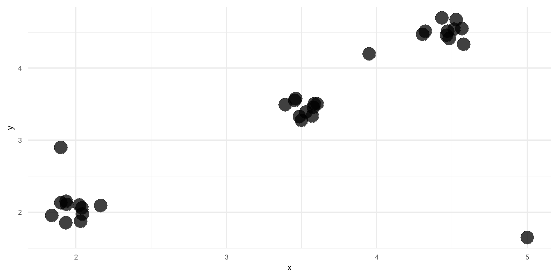
4.1 Toy data

聚类前后对比

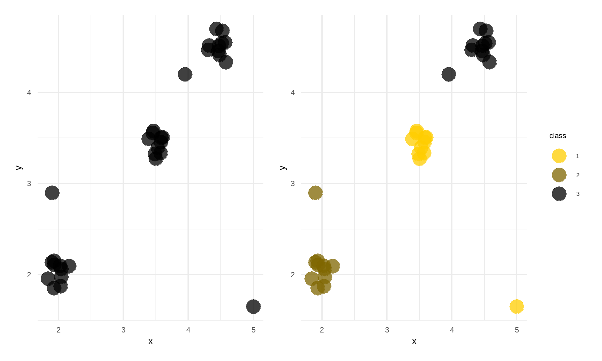
4.2 层次聚类 (Hierarchical clustering)

Agglomerative vs. Divisive

• Agglomerative (/ə’ɡlɔmərətiv/) 基于 a wide variety of similarity measures，从empty graph （没有任何ties）开始，将最similar的nodes加在一起
• Divisive 从complete graph 开始， dedrogram横切二分点）（halting points）

A善于发现强连结community， D不会去除peripheral vertices；类似EFA和PCA的差别

4.3 层次方式方法与标准

常见分类（叉）linkage

• Single-linkage
• Complete-linkage
• Average-linkage
• Centroid-linkage
• Ward’s minimum variance method

分类（叉）标准 （\(d(a,b)\) \(a\) 和 \(b\) 之间的距离）

• Single-linkage: \(\min \{ d(a,b):a\in A, b\in B \}\)
• Complete-linkage: \(\max \{ d(a,b):a\in A, b\in B \}\)
• Average-linkage: \(\frac{1}{|A||B|}\sum_{a\in A}\sum_{b\in B}d(a,b)\)
• Centroid-linkage: \(||c_t - c_s||\), where \(c_s\) and \(c_t\) are the centroids of clusters \(s\) and \(t\).

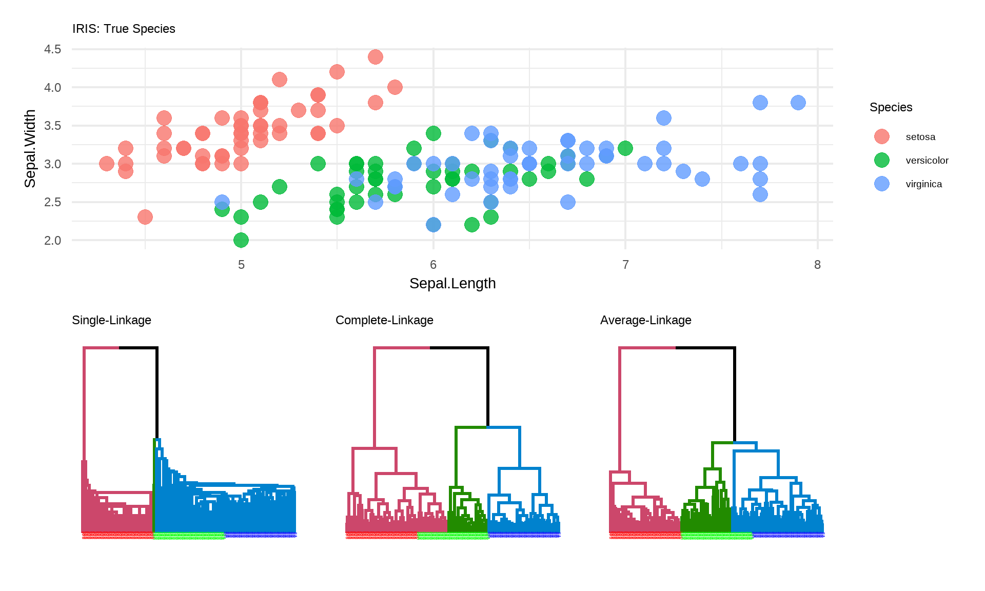
4.4 常见 Linkages 比较

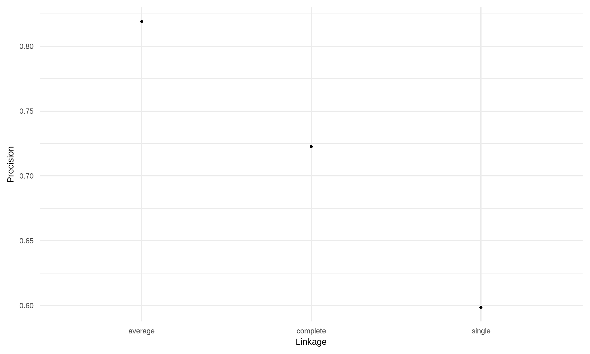
4.5 三种linkages的精确度

4.6 非层次聚类 (Non-hierarchical clustering)

• Centroid-based： K-means, K-medians, K-medoids, K-modes……
• Model-based: Gaussian, gamma, t, poisson, GMM……
• Density-based
• Grid-based

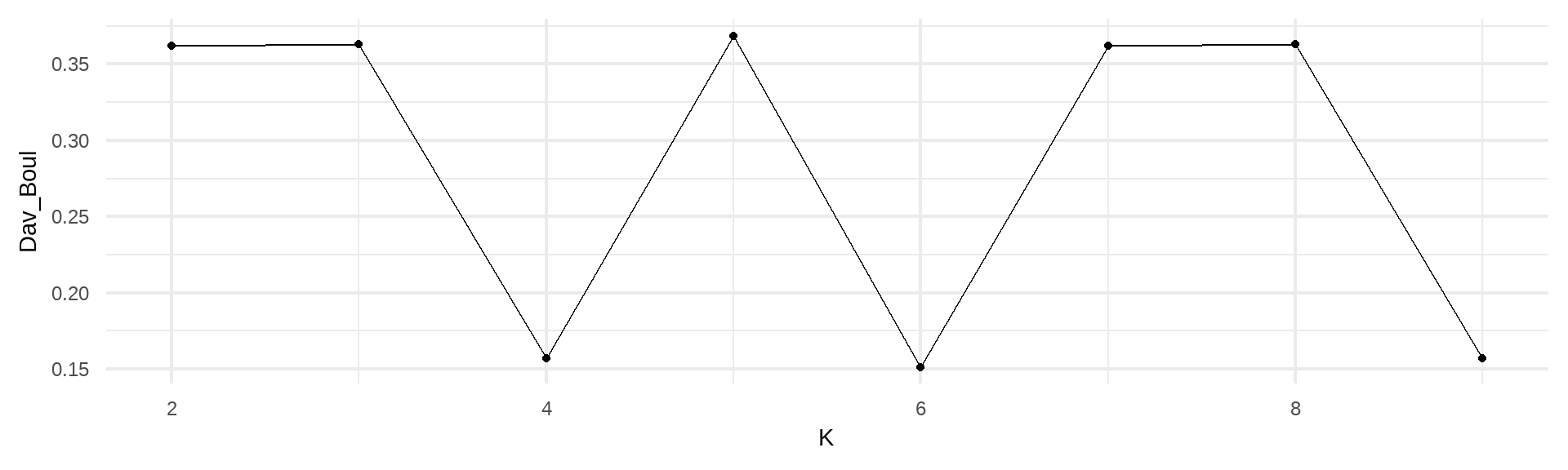
4.7 聚类之前：聚几类？

基本思路

\[ Max(\frac{类内相似性}{类间相似性}) \]

常见标准：

• Silhouette
• Davies-Bouldin index
• Dunn index

判断方法：¹

5个是最佳的选择，不过为了显示方法差别，后面采用3个

1. 与EFA判断方式一样（为什么？）

4.8 Centroid-based: K-Mean

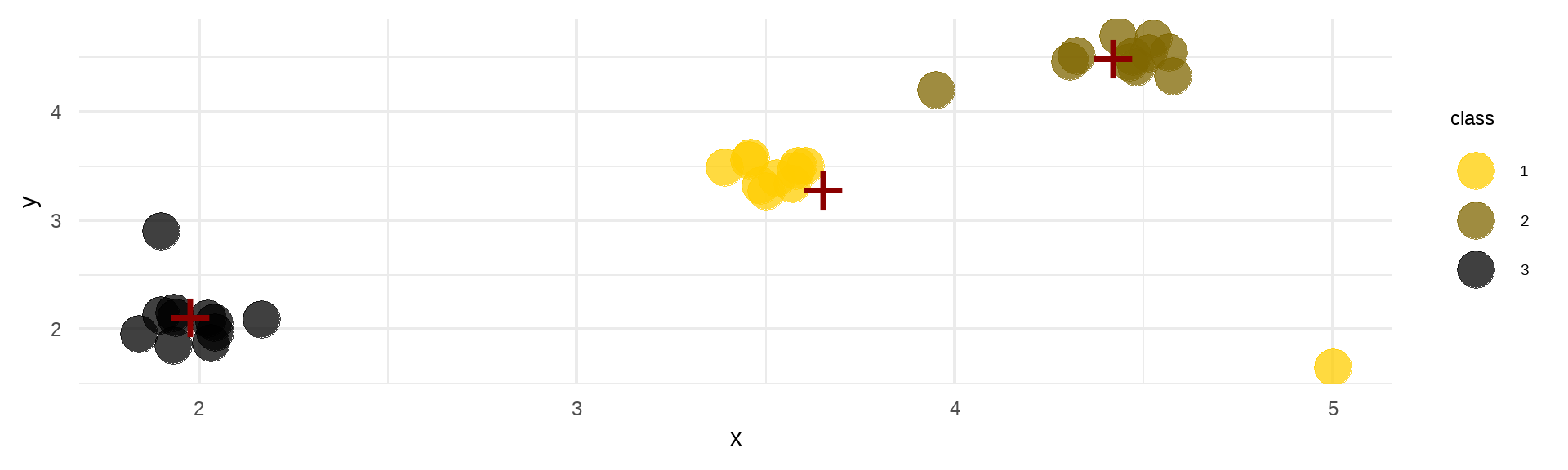
步骤

1. 创建随机的K个聚类（并计算质心）。
2. 将点分配给最近的质心。
3. 更新质心。
4. 当质心仍在变化时，返回步骤2。

优点：计算速度快。易于理解

缺点：

• 初始值敏感
• 量纲敏感
• 只能创建凸形聚类
• 对异常值敏感

4.9 Centroid-based: K-medoids

使用中心点而非平均值

优点

• 对异常值不太敏感
• 可以使用任何距离度量

缺点

• 初始值敏感
• 量纲敏感
• 比K-means算法慢

Medoids: the one that minimizes the total distance to all other points，a real one not a calculated mean

4.10 Centroid-like: Spectral Clustering

基于谱分解（spectral decomposition）提取数据特征，然后根据特征聚类。¹

步骤：

1. N = 数据数量，d = 数据维度，
2. \(\mathbf{A}\) = 相似度矩阵，\(A_{ij} = \exp(- (data_i - data_j)^2 / (2*\sigma^2) )\) - N × N矩阵，
3. \(\mathbf{D}\) = 对角矩阵，其(i,i)元素是\(\mathbf{A}\)第i行元素之和 - N × N矩阵，
4. \(\mathbf{L}\) = \(\mathbf{D}^{-1/2} \mathbf{A} \mathbf{D}^{-1/2}\) - N × N矩阵，
5. \(\mathbf{X}\) = \(\mathbf{L}\)的k个最大特征向量的集合 - N × k矩阵，
6. 将\(\mathbf{X}\)的每一行归一化为单位长度 - N × k矩阵，
7. 在\(\mathbf{X}\)上运行K-means算法。

1. 虽然使用到了k-mean，但之前步骤导致两种方法的数学基础有本质不同。

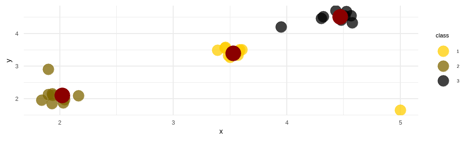
4.11 谱聚类效果

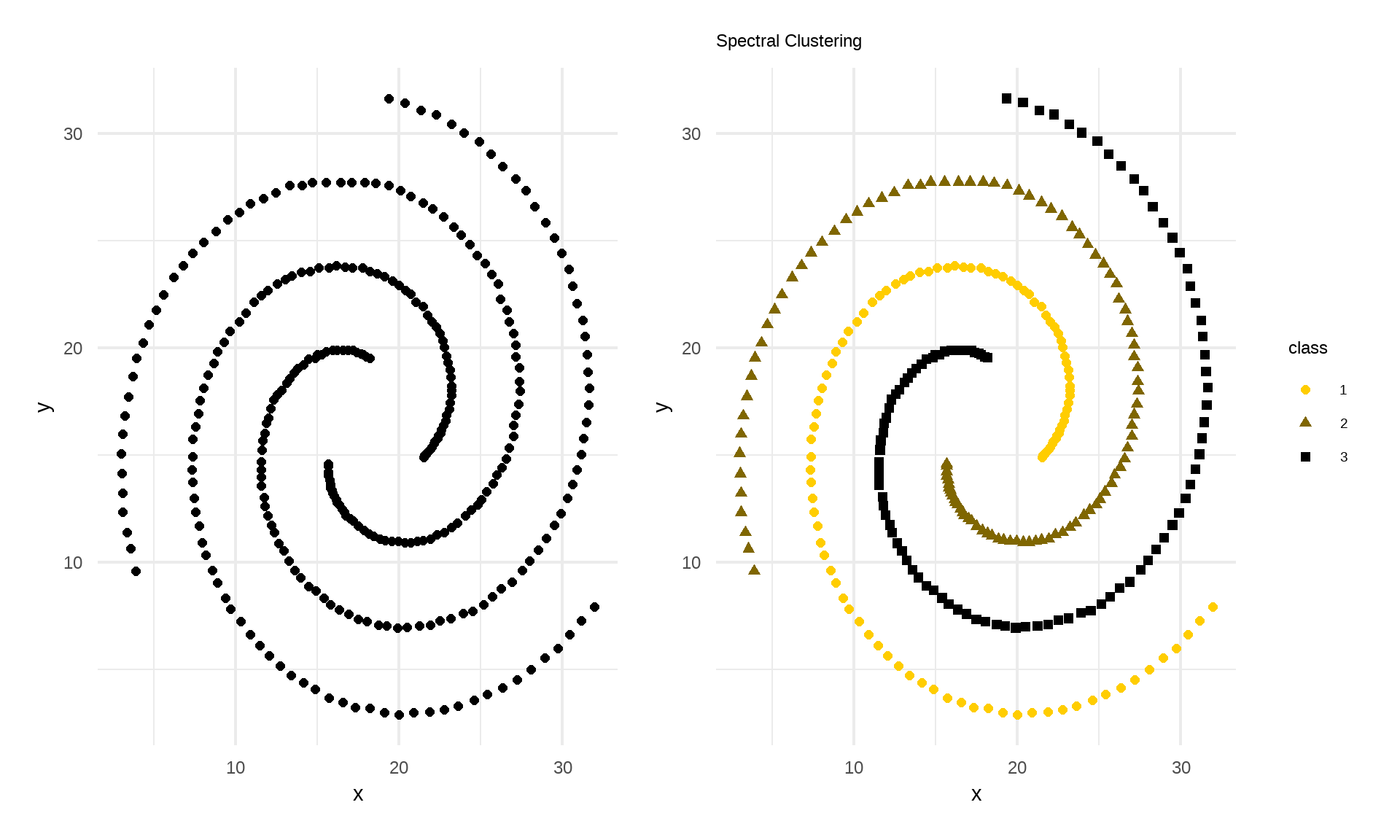
4.12 Model-based: GMM

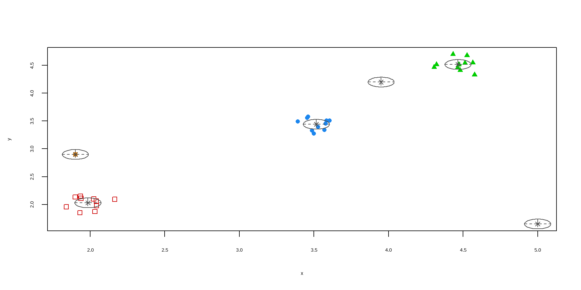
通常对于多维数据采用Mixture of models, 比如Gaussian Mixture Models (GMM)

\[ L(\boldsymbol{\mu_1}, \dots, \boldsymbol{\mu_k}, \boldsymbol{\Sigma_1}, \dots, \boldsymbol{\Sigma_k} | \boldsymbol{x_1}, \dots, \boldsymbol{x_n}). \]

Cluster: mean (\(\mathbf{\mu}\)) and covariance matrix (\(\mathbf{\Sigma}\)) Here, cluster is represented by . So not just centroid as in the case of K-means.

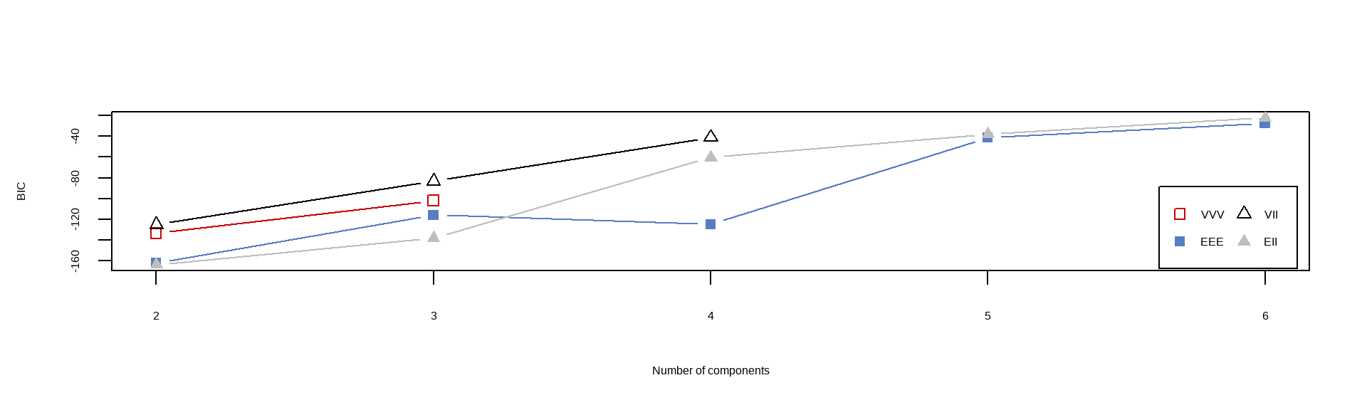
类数选择：BIC

4.13 操作过程

• 目标：Maximum likelihood
• 过程：Expectation Maximization (EM)

4.14 Density-based 方法

定义密度，然后寻找最大化密度的点

常见方法:

• DBSCAN: 用neighborhood定义密度，所有点必须在一定距离内，每个cluster里必须有一定数量的点¹
• OPTICS
• HDBSCAN
• Multiple densities (Multi-density) methods

优点

• 自动提取异常值
• 计算速度快
• 可以找到任意形状的簇
• 根据数据自动确定簇的数量

缺点

• 必须预设参数（\(\epsilon\)，minPts）值
• 邻域可能存在连接问题

1. 未与任何cluster连接且未通过最小点标准的点被标记为噪声（异常值）

4.15 DBSCAN效果

4.16 DBSCAN优势

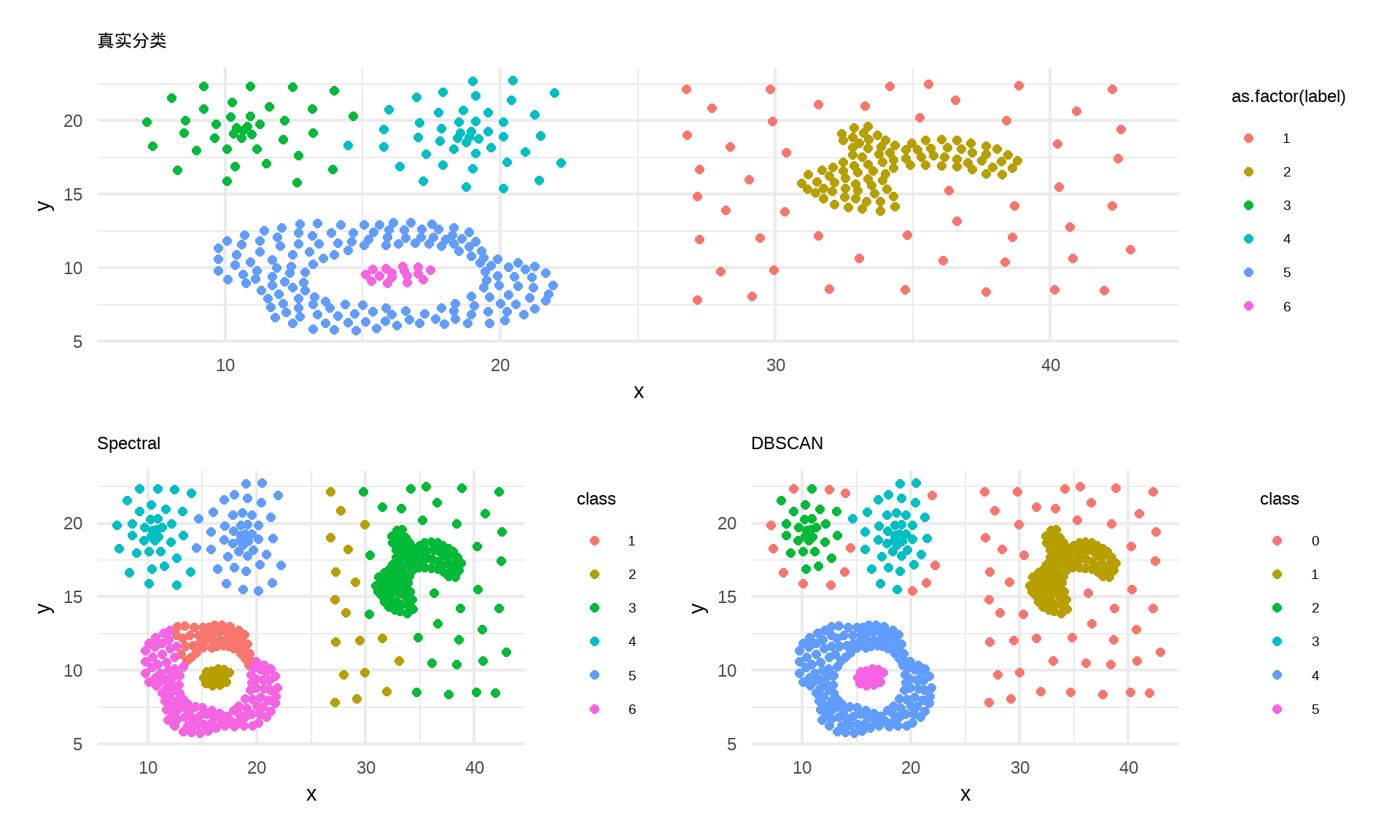
4.17 DBSCAN vs. Spectral

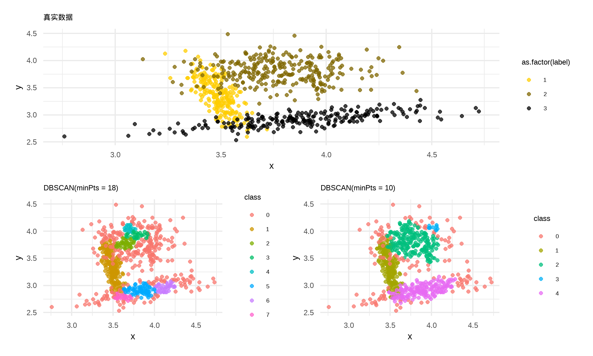
4.18 初始值影响DBSCAN效果（交叠数据聚类）

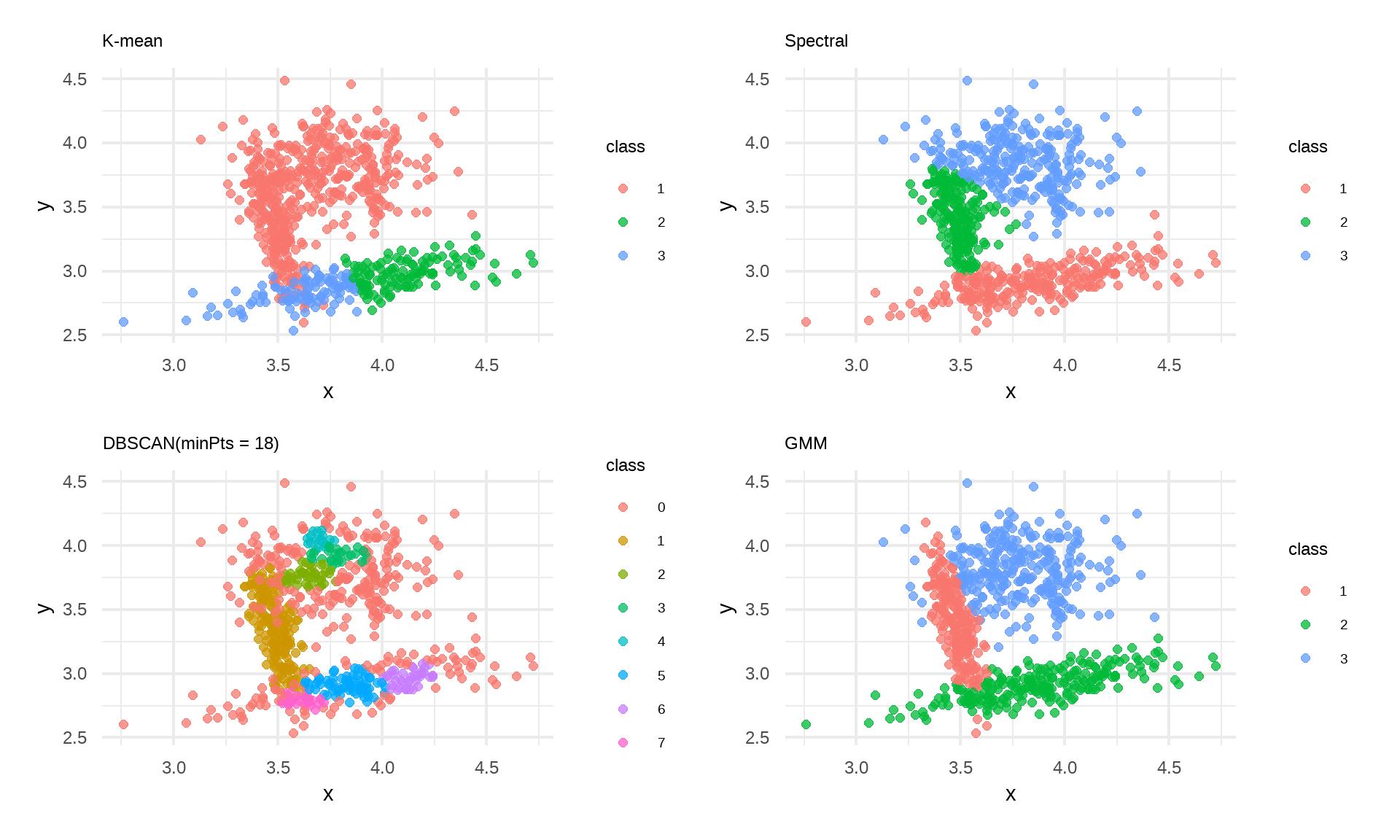
4.19 方法对比

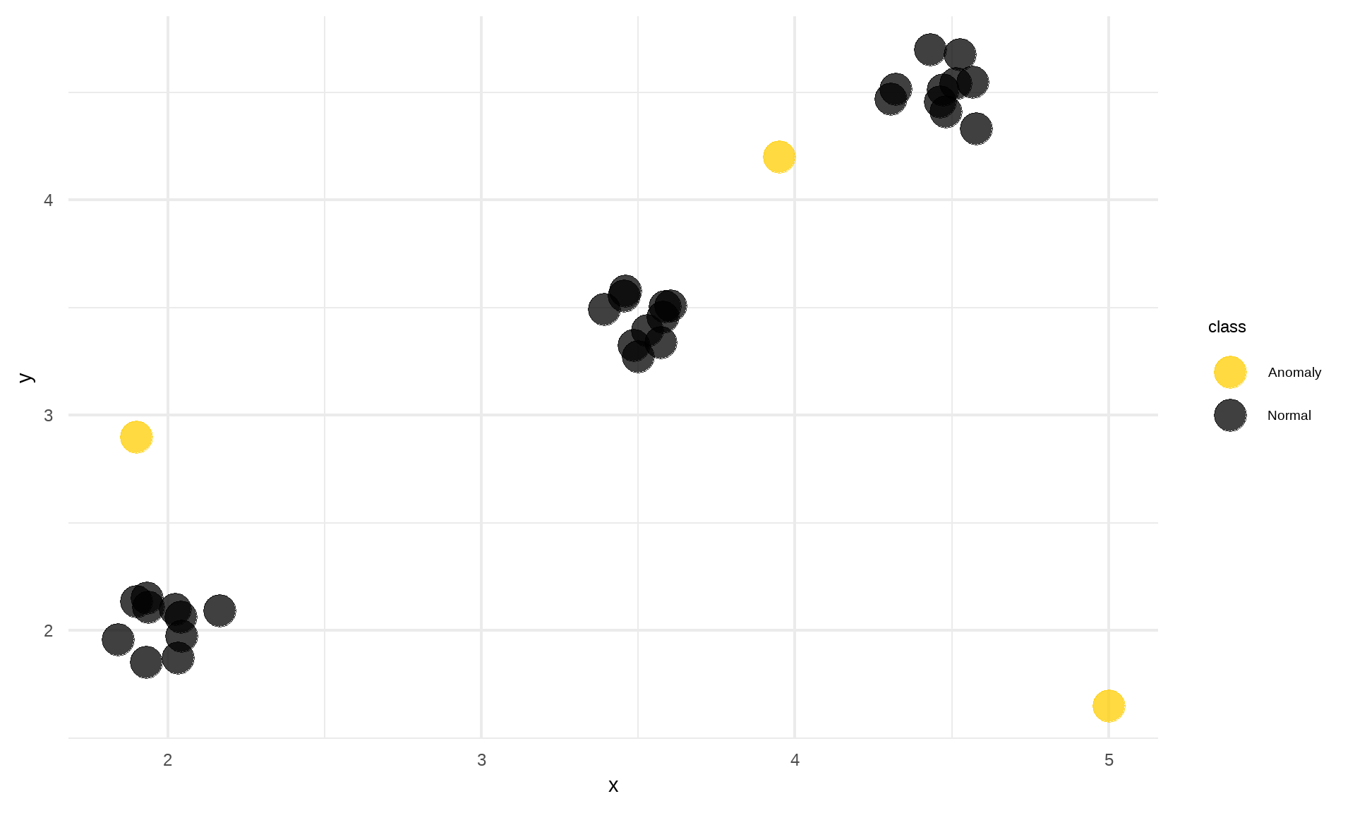
4.20 聚类除了聚类以外的功能

甄别异常值

数据浓缩/降维

5 附录：全网分析

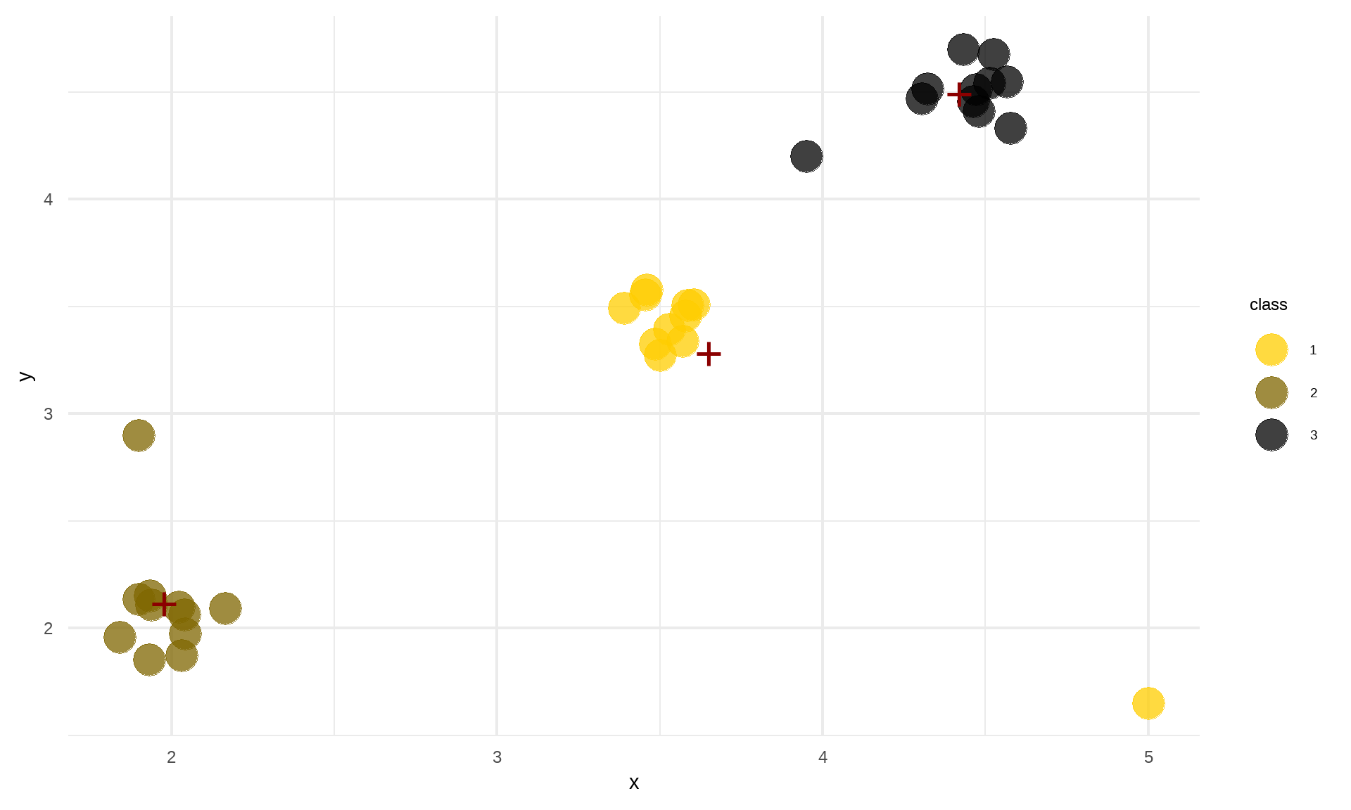
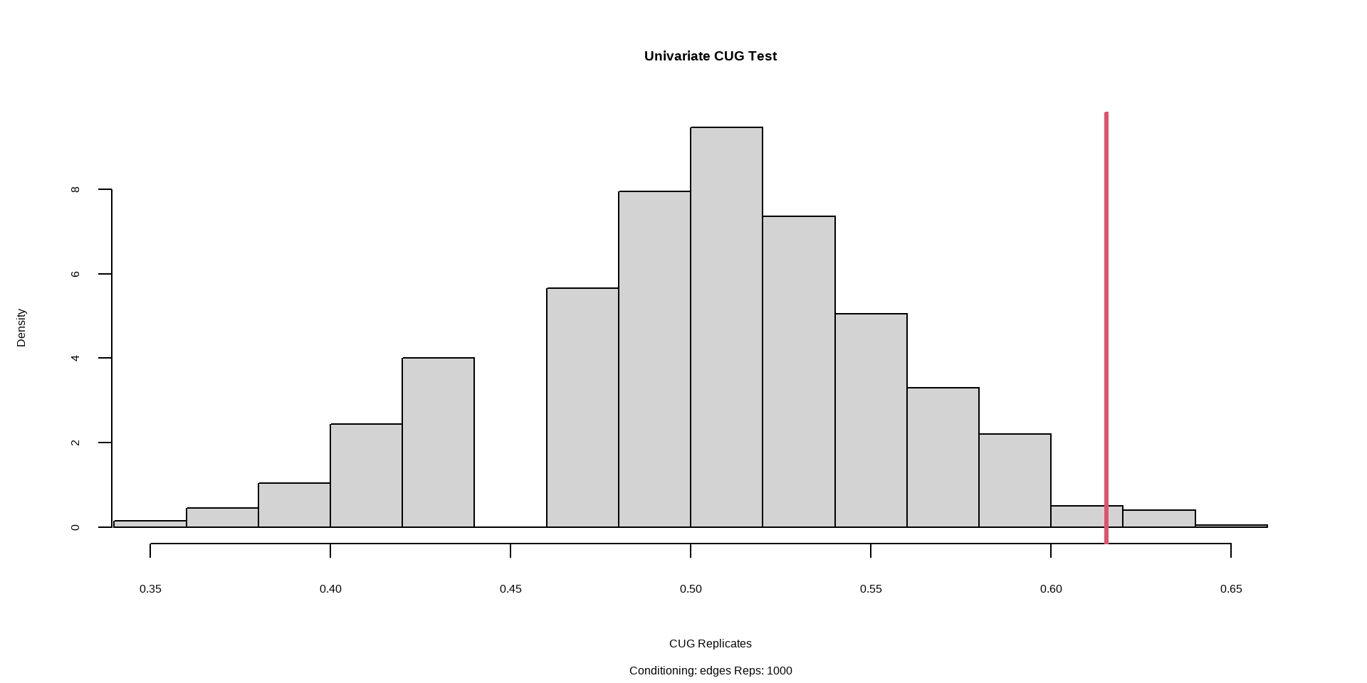
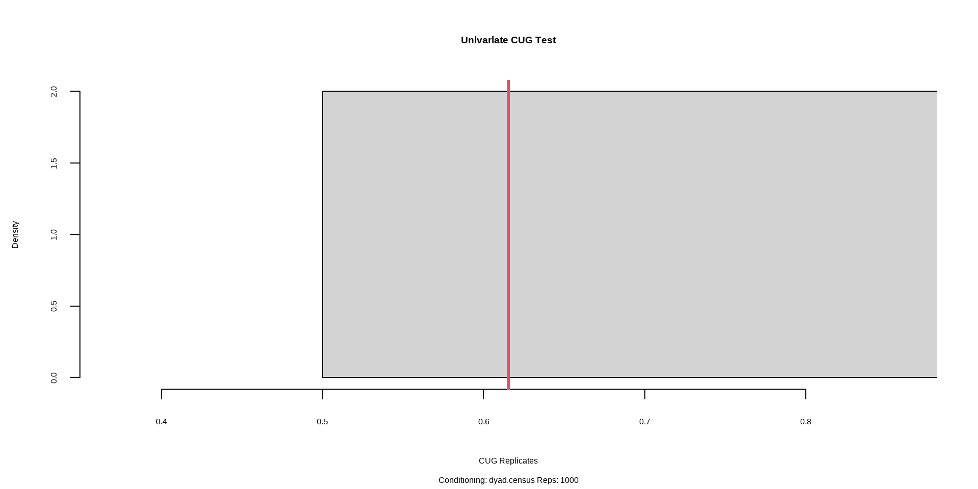
5.1 CUG

“Baseline network”比较分析的一种

1. 固定属性 (size, prob of edges, dyad census, degree, # of triangles, etc.)
2. 同等可能

根据特定属性通过bernoulli分布建立随机网络，所有网络都是被视为同等可能出现

• n: The size of the vertex set (|V(G)|) for the random graphs
• m: The number of graphs to generate
• tprob: Information regarding tie (edge) probabilities; see below

Generating 1000 random graphs of size 20; assumes digraph. tprob, probability of any tie existing is 30%. Plotting the density. it is probability, so, some is before 0.3, some beyond 0.3

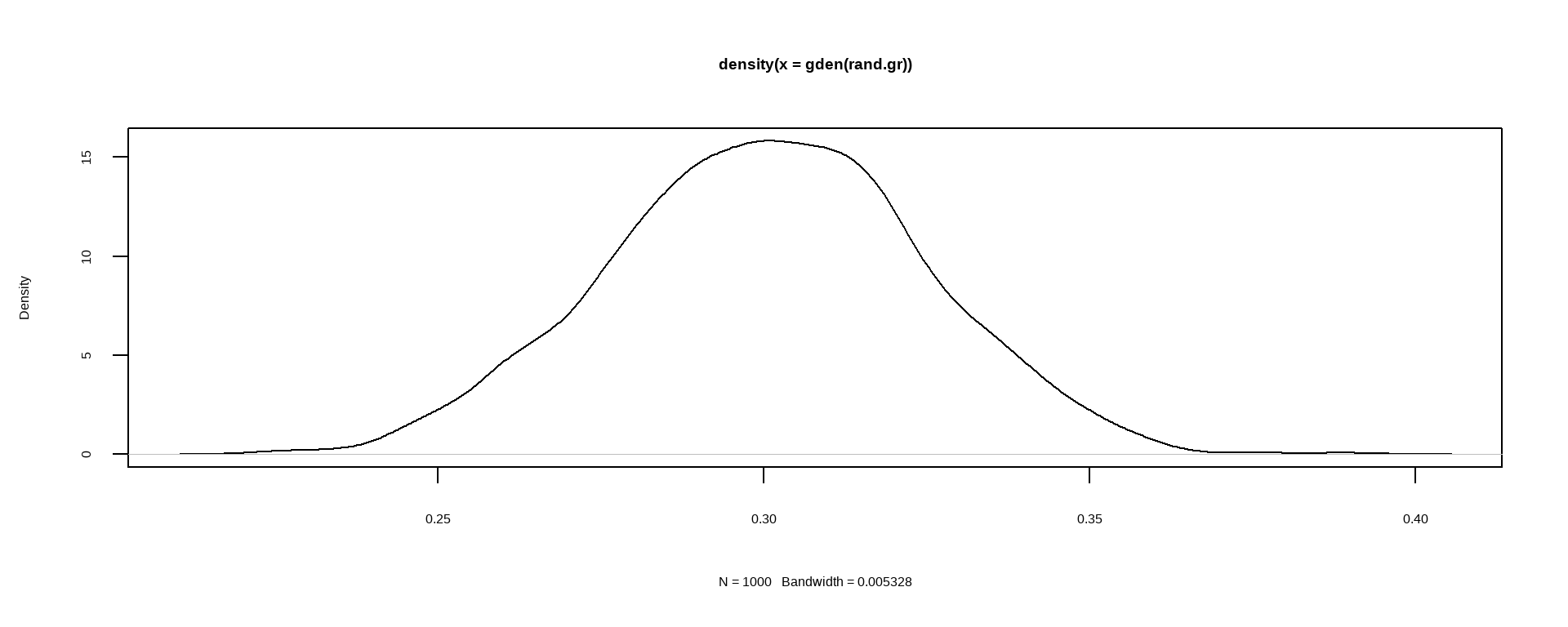
5.2 H₀

\[ Network_{obs}\quad vs.\quad Network_{ran} \]

观测网络与随机网络在这些方面是否相异

5.3 Conditional Uniform Graph Test

Density

Density

Edge

Dyad Census

Drabek et al. (1981) provide seven case studies of emergent multi-organizational networks (EMONs) in the context of search and rescue (SAR) activities. Networks of interaction frequency are reported, along with several organizational attributes.

Drabek等人（1981年）提供了七个关于搜救（SAR）活动中涌现的多组织网络（EMONs）的案例研究。报告了互动频率网络，以及几个组织属性。

5.4 QAP

• 创建随机网络分布 (= CUG)
• 控制网络结构 (≠ CUG)

网络结构: centrality 等

non-parametric，从sample中抽出两组，对比stats，看是否一样。 与t-test等的对比重要不同在于不是跟normal比

通过permutation test实现:

1. 计算原始网络的correlation coefficient;¹
2. Permute一些vertices；
3. 将Permuted 网络和原始网络相对比；
4. 一顿狂Permute + 狂比
5. 看看correlation的分布
6. 确定特定值和原始网络相同的概率

网络correlation 根据两点除相互连接外的其他degree (remaining degree)计算

1. Pearson’s r correlation or Euclidean distance

5.5 多元网络分析 (QAP)

OV: 网络
EV: 解释变量adjacency matrices

\[ E(\text{Advice}_{ij}) = \beta_0 + \beta_1\text{Reports}_{ij} + \beta_2\text{Friends}_{ij} +... \]

Network Logit Model

Coefficients:
            Estimate   Exp(b)     Pr(<=b) Pr(>=b) Pr(>=|b|)
(intercept) -0.4251826  0.6536504 0.4     0.6     0.4      
x1           0.5794452  1.7850479 1.0     0.0     0.1      
x2           3.0589826 21.3058690 1.0     0.0     0.0      

Goodness of Fit Statistics:

Null deviance: 582.2436 on 420 degrees of freedom
Residual deviance: 548.1452 on 417 degrees of freedom
Chi-Squared test of fit improvement:
     34.09844 on 3 degrees of freedom, p-value 1.888613e-07 
AIC: 554.1452   BIC: 566.266 
Pseudo-R^2 Measures:
    (Dn-Dr)/(Dn-Dr+dfn): 0.07509042 
    (Dn-Dr)/Dn: 0.05856387 
Contingency Table (predicted (rows) x actual (cols)):

         Actual
Predicted     0     1
        0   188   122
        1    42    68

    Total Fraction Correct: 0.6095238 
    Fraction Predicted 1s Correct: 0.6181818 
    Fraction Predicted 0s Correct: 0.6064516 
    False Negative Rate: 0.6421053 
    False Positive Rate: 0.1826087 

Test Diagnostics:

    Null Hypothesis: qap 
    Replications: 10 
    Distribution Summary:

       (intercept)       x1       x2
Min       -4.50574 -2.69571 -1.40610
1stQ      -3.92006 -0.19556 -0.04667
Median    -3.25925  0.08638  0.52835
Mean      -3.28825  0.08504  0.33152
3rdQ      -2.73010  0.67105  0.86806
Max       -2.09563  2.38630  1.15204

There are also netlm etc.

Not 10, often over 1000

null hyp choices: qap quick, qapspp robust

5.6 ERGM沿革

Simple Random Graph Model

↓

P¹ Model

↓

P^* Model

↓

ERGM &rarr GEGM/TEGM…

5.7 Simple Random Graph Model

\[ P(X = x) = \frac{exp(\theta_LL(x))}{k(\theta)}. \]

• L: # of arcs
• θ: edge parameter¹

1959，只允许specify links

Bernoulli Assumption

• Tie 是独立的（🤨）
• IID ties → Log-probability of a graph is proportional to a weighted sum of edge-count

基于这个assumption才有simple random graph

1. k(θ)意在标准化, 整个结果和为1。

5.8 P¹ Model

\[ P(X = x) = \frac{exp(\theta_LL(x) + \color{red}{\theta_MM(x) + \sum_i\alpha_iy_{i+} + \sum_j\beta_iy_{+j}})}{\kappa(\theta)}. \]

• M: # of mutual
• y_i+: # outgoing ties
• y_+j: # incoming ties

Bernoulli Dyad Independence Assumption

• 允许互惠和不同方向的不同作用
• 用于binary,有向网络

• Allows for reciprocity and differential attractiveness
• Useful for binary, directed graphs

所有高于degree of reciprocity的性质都不能解决, 没人再用

5.9 P^* Model

\[ P(X = x) = \frac{exp(\sum_i\theta_i\color{red}{z_i(x)})}{\kappa(\theta)}. \]

z_i: any network statistics加在一起

Dyad Independence Markov assumption

• Ties are (conditionally) independent unless they share a node.
  • Parallels in Markov chains, time series, spatial analysis
• Think of nodes as connecting edges to obtain this dependence structure
• Ties are conditionally dependent if and only if they share a node

ERGM基于此发展而来，现在两者区别更多是computational而非想法上的

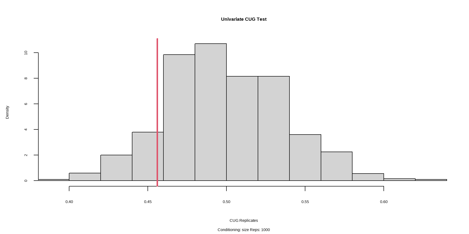
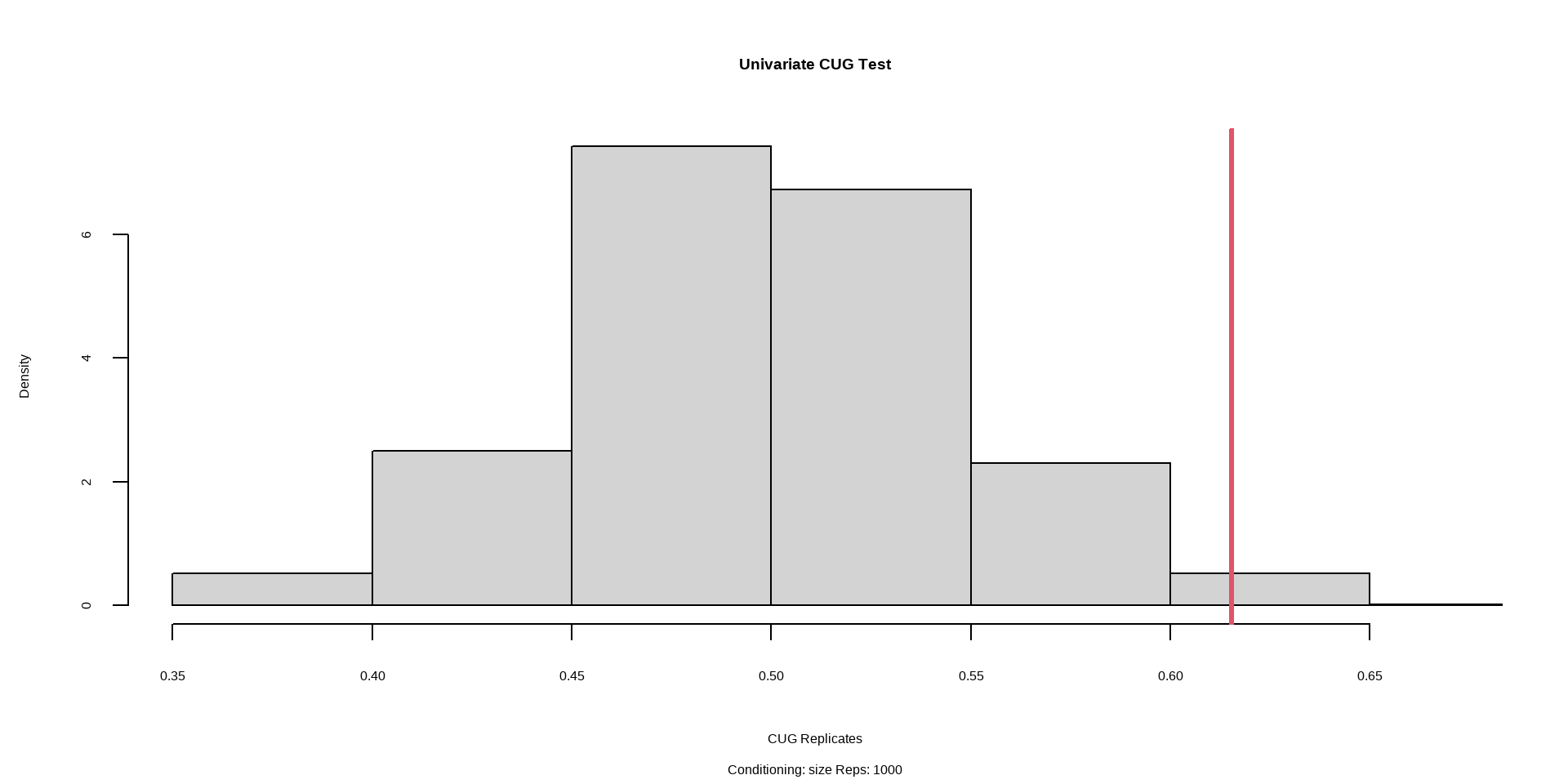
5.10 Network Statistics

Things one can test in P*, path closure: 多重triangle

算起来更麻烦， necessary

如果你想了解更多

GOOGLE上没有全的表

5.11 理解ERGM结果

\[ P(N, \boldsymbol{\theta}) = \frac{exp(\boldsymbol{\theta'h}(N))}{\sum_{N^*\in N}exp(\boldsymbol{\theta'h}(N^*))}. \]

• Network level：exp(θ)，relative likelihood of observing Nⁱ⁺ to observing N^i-

增加一个network statistics 比不加它变化的likelihood

odd-like stuff: 那么 θ = 0代表什么？

θ = 0 ⇒ exp(θ) = 1 ⇒ 增加或不增加这个stats看到observed network几率是一样的，a.k.a., 没用

• Edge level：exp(θ_rδ_r^(ij)), P(N_ij = 1|N_-ij, θ) = logit^-1∑_r=1θ_rδ_r^(ij)(N)

δ_r^(ij): Change parameter

记录改变多少： 比如同样是增加一个edge，对于mutual（包含reciprocal和not conntected），对于i 和 j已经相连的情况，加一个edge是增加了一个mutual，那么δ + 1, 但如果i 和 j不相连，那么加一个edge，是把一个互不相连的mutual弄没了，δ - 1。 所以实际计算比较复杂，但btergm::interpret

\(logit^{-1} = frac{1}{1 + e^{-1}}\)

• Nodal level: Block-wise conditional distributions

Blocks are split according to an attribute, complicated

5.12 跑完不算完

诊断

• Convergence
• Degeneracy

Super important!

Degenracy is ERGM goodness of fit, unstable results, random process, model fit, little changes a lot; leading to prediction that everyone should connect to everyone or none

Looking for high p-value (not violate the assumptions)

Convergence is for Markov Chain

局限

1. MPLE vs. MLE vs. MCMC-MLE
2. Degeneracy
3. Sensitivity to missing data

1. Maximum pseudo LE； 前两个对P1之前还好，之后算不出来

Theory really matters!! 来解释要加什么network statistics

怎么解决 geometrically weighted degree distribution

1. Sensitivity

发展

• GERGM
• TERGM
  • STERGM
• FERGM

……

G ERGM: weighted ergm

S TERGM: Network panel data, Separable TERGM for each time point the ties formatting and disoluting independently

F ERGM: Frailty ERGM “individual-level random effects” for the propensity for a directed tie

5.13 Network analysis 🤝 Spatial Analysis

Modeling Peer Influence

\[\begin{align} \boldsymbol{Y}^{(1)} &= \boldsymbol{XB},\\ \boldsymbol{Y}^{(t)} &= \alpha\boldsymbol{WY}^{t} + (1 - \alpha) Y^{(1)}. \end{align}\]

• Y⁽¹⁾: N个人，每人对M个问题的初始看法 (N × M);
• X: K个会影响个体看法的（外生性）变量（N × K）;
• α: （内生性的）人际影响对Y的作用的比重;
• W: 人际关系矩阵（N × N).