持续时间分析

政务大数据应用与分析 (80700673)

胡悦

清华大学社会科学学院

概要

今天，让我们成为生物学家

• 持续时间分析概念
• 持续时间分析模型

1 持续时间分析

1.1 什么是持续时间数据

• 数据类型
  • 什么时候开始/结束
  • 延续了多久？
  • 需要多久才能发生？

• 之于大数据
  • （某种意义上）最常见的大数据类型
  • 社交媒体分析
  • 司法数据分析
  • 体育数据分析
  • 政务数据分析
    ……

Terminology

• Survival analysis
• Event history analysis (discrete)
• Failure analysis
• Duration analysis (continuous)
• Frailty (e.g., engineer)
• Cure models (e.g., medical)

Frailty /fr’eɪlti/ 弱点脆弱

1.2 持续时间数据本质

在分析前要想清楚的

• 解释变量对事件的影响方式？
• 事件是否被视为重复的？
• 发生周期（duration）是否时完全可见的？
• 事件分布（event rate）如何在时间维度上变动？

⇓

策略选项

1. Count：发生了多少次
2. Discrete：年、月、天；0s & 1s.
3. Duration: 具体时长

2 Counting model

2.1 Counting data

就是字面意思，count出来得数据。

1. 每周网络故障次数
2. 每小时网站访问者数量
3. 餐厅到达的顾客数量
4. 每小时呼叫中心接到的电话数量
5. 城市平均风暴次数
6. 医院每分钟接到的紧急呼叫数量

与连续变量的不同

1. 离散
2. 非负 (0，+∞)
3. 有有意义的0

PMF: \(Pr(X{=}k)= \frac{\lambda^k e^{-\lambda}}{k!},\)

k is the number of occurrences

μ = σ² = λ.

&lambda is the average rate of occurrence

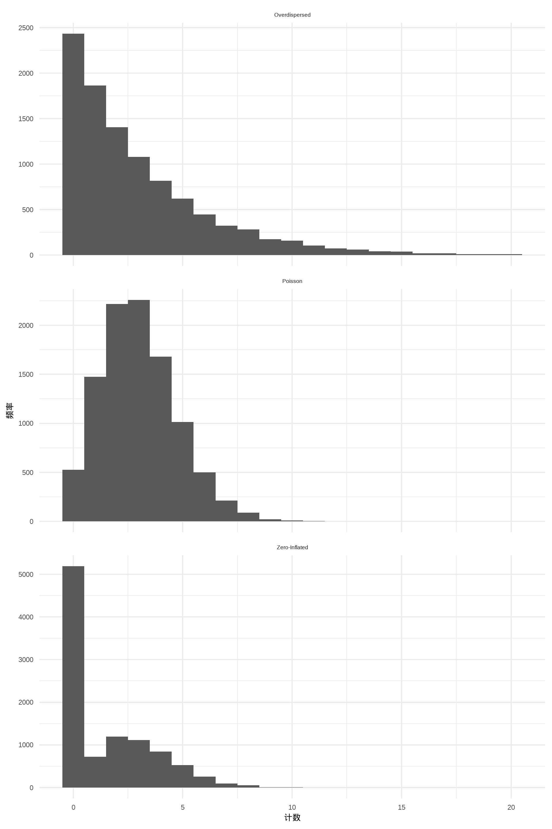
2.2 Overdispersion & Zero-Inflation

解法

1. Negative Binomial \[\Pr(X=k)={\binom {k+r-1}{k}}(1-p)^{k}p^{r},\]
   • r: number of successes
   • k: number of failures
   • p: probability of success on each trial.
2. Zero-Inflated Models/hurdle model

ZIMs are particularly useful when the data include excess zeros but also a meaningful count distribution among the non-zero observations. Hurdle models are more suited for situations where the non-occurrence of an event (zero counts) and the occurrence (positive counts) are thought to arise from different processes

3 Discrete Model

3.1 事件史分析

关注事件发生点，解释与何因素有关，通常被称作“事件史”（event history）分析。

分析前认知：

1. 何时开始计时
2. 如何判定事件发生

主要步骤：

1. 结果变量：通常该变量在事件发生时记为1，之前均为0
2. 解释变量：在每个时间点均有记录

虽然分析中各事件看起来是同时开始的，但其实不然

当事件发生后，该观测单元将不再存在于risk set中。

3. 估计
   • Risk set： 在给定时间点上，观测单元触发事件的可能性, \(R(t)\equiv \{i, y_{it} = 0 | y_{it} = 1\}.\)

unit	time	event	ev	risk
1	1	0	4.3	1
1	2	0	1.2	1
1	3	1	4.2	1
1	4	NA	1.6	0
2	5	0	6.1	1
2	6	0	3.2	1
2	7	0	7.2	1
2	4	1	3.9	1

公式预警

公式对于理解持续时间分析非常之重要!🥁🥁🥁

3.2 结果变量分布

Survival rate: the probability that an event will continue to exist (\(T\)) beyond a certain period of time (\(t\)).

\[S(t|X) = P(T > t | X).\]

PDF: \(f(t|x) = P(T = t | X).\)

CDF: \(F(t) = P(T\leq t | X) = 1 - S(t).\)

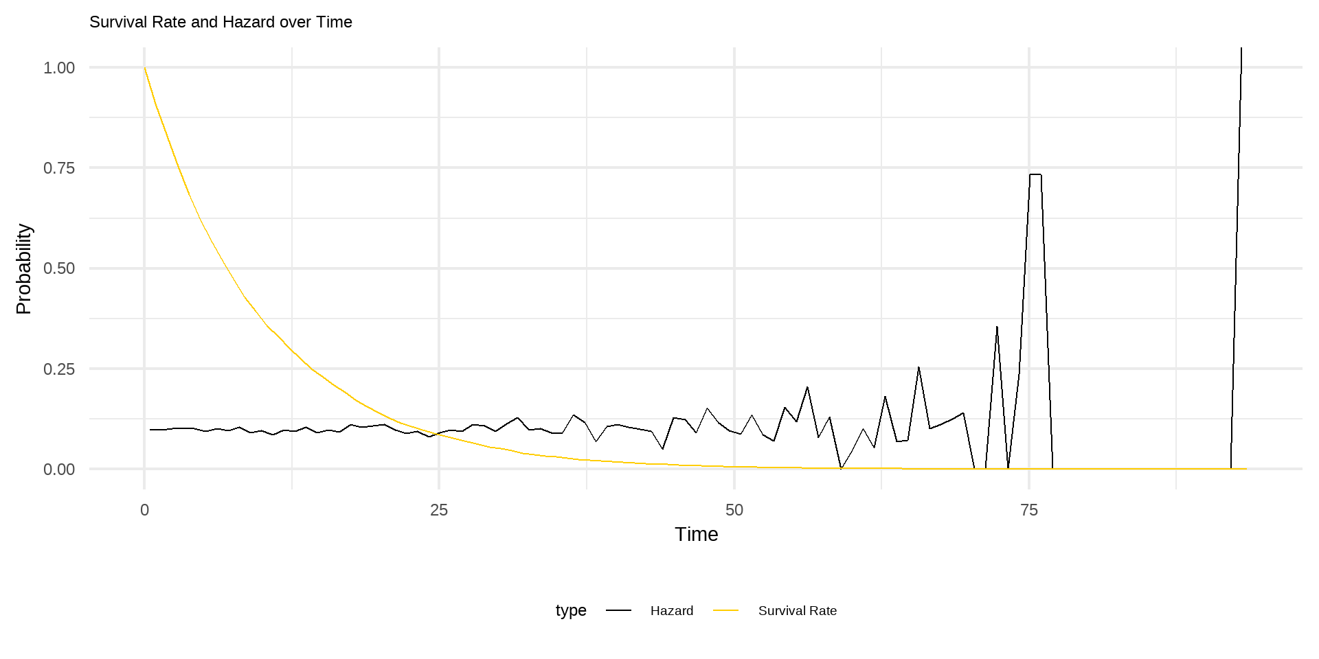
Hazard: the instantaneous risk at that time of the event happening, given that it hasn’t happened yet.

\[P(T = t|T\geq t, X) = \frac{f(t|X)}{S(t|X)} = \frac{P(T \color{red}{=} t | X)}{P(T \color{red}{>} t | X)}.\]

Hazard: the probability that the event occurs during a specific time point, given that it hasn’t already occurred.

3.3 Hazard

The probability that the event occurs during a specific time point, given that it hasn’t already occurred.

It’s like watching a tightrope walker crossing between two skyscrapers. The hazard is the risk of falling at any given moment during the walk, considering the walker hasn’t fallen yet.

Example of Hazard in Real Life:

Light Bulbs: Suppose we find that the hazard of a particular brand of light bulbs increases significantly after 1,000 hours of use. This means the risk of these bulbs burning out gets much higher beyond this point.

Patients in a Clinical Trial: If we’re studying a new medication, the hazard might represent the risk of a patient having a side effect at any given time during the study, assuming they haven’t experienced it yet.

3.4 Hazard vis-a-vis Survival Rate

This graph shows the rate at which the event of interest is expected to occur at different times, given that it hasn’t occurred yet.

3.5 事件史分析工具

• logit/probit
• c-log-log
• scobit
• expit

c-log-log: complementary log-log, \(\eta(x) = \log(-\log(1-\pi_x))=\mathbf{x}\beta\)

scobit: skewed logit

expit: exponential logit

3.6 Logit/Probit模型

• logit/probit
• c-log-log
• scobit
• expit

令 \(Y^*\) 为导致可见事件( \(Y_{it}\) )发生的不可见变量：

\[ Y_{it} = \begin{cases} 1 & \text{if } Y^*\geq 0, \\ 0 & \text{if } Y^*< 0. \end{cases} \]

那么

\[ \begin{align} P(Y_{it} = 1|X) =& P(Y^* \geq 0|X)\\ =& P(X\beta + \epsilon\geq 0|X)\\ =& P(\epsilon\geq 0 - X\beta|X)\\ =& 1 - P(\epsilon\leq - X\beta|X)\\ =& 1 - F(-X\beta|X) \end{align} \]

3.7 Logit模型

令 \(\epsilon\sim logistic\),¹ 则 \[P(Y_it = 1|X) = 1 - \Lambda(-X\beta) = \Lambda(X\beta).\]

代入logistic分布可得，

\[ \begin{align} P(Y_{it} = 1|X) =& 1 - \frac{e^{-X\beta}}{1 + e^{-X\beta}}\\ =& \frac{e^{X\beta}}{1 + e^{X\beta}}\\ P(Y_{it} = 0|X) =& \frac{1}{1 + e^{X\beta}} \end{align} \]

\(\beta_{probit} = \frac{\sqrt 3}{\pi}\beta_{logit}.\)

此处用probability来建构likelihood, 因为likelihood存在scale issue, 通常不可知。此法被Gary称为Unified Maximum Likelihood

1. 对于probit，则令 \(\epsilon\sim i.i.d. N(0, 1)\), 则 \(P(Y_it = 1|X) = 1 - \Phi(-X\beta) = \Phi(X\beta).\)

3.8 应用举例

研究美国印第安部落与州协调法案（Indian Gaming Compact）推行情况

解释变量：

• Religion (religion), the number of federally recognized tribes (fedtrib)
• Total population (totpop)
• Real income per capita (rpcpinc)
• Ideology score (ideology)
• Federal government recognized tribes (fedtribe)

原始数据

state	stateno	year	totpop	rpcpinc	ideology	fedtribe	religion	adopt_year
AL	1	1989	4.102	18.02829	-23.1	1	33.9	NA
AL	1	1990	4.118	17.85045	-23.1	1	33.9	NA
AL	1	1991	4.087	18.02460	-23.1	1	33.9	NA
AL	1	1992	4.131	18.56343	-23.1	1	33.9	NA
AL	1	1993	4.181	18.66846	-23.1	1	33.9	NA
AL	1	1994	4.215	19.08401	-23.1	1	33.9	NA

3.9 建立Risk set

\(R(t)\equiv \{i, y_{it} = 0 | y_{it} = 1\}.\)

在给定时间点观测单元触发事件的可能性, 对于一个周，没推行是1，推行了则被减去

可分析数据

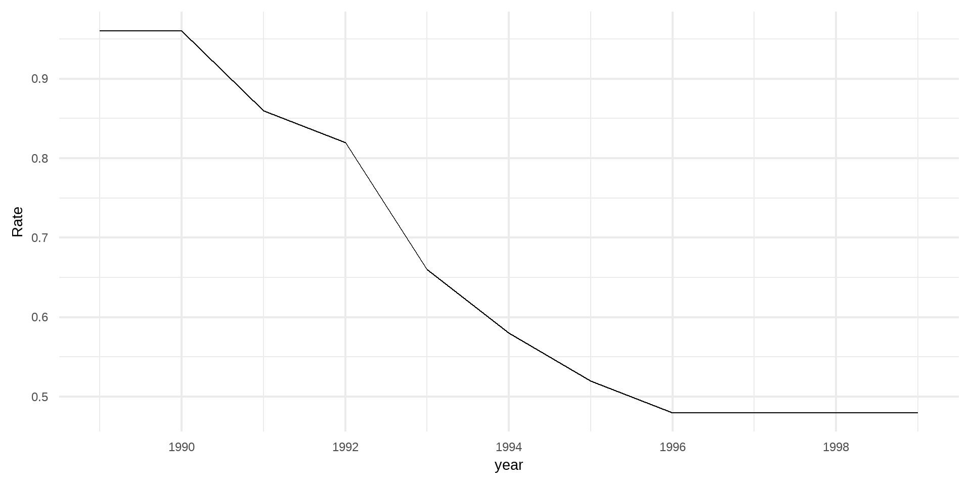
year	sum_adopt	sum_risk	hazard	survival
1989	0	48	0.00	0.96
1990	5	48	0.10	0.96
1991	2	43	0.05	0.86
1992	8	41	0.20	0.82
1993	4	33	0.12	0.66
1994	3	29	0.10	0.58
1995	2	26	0.08	0.52
1996	0	24	0.00	0.48
1997	0	24	0.00	0.48
1998	0	24	0.00	0.48
1999	0	24	0.00	0.48

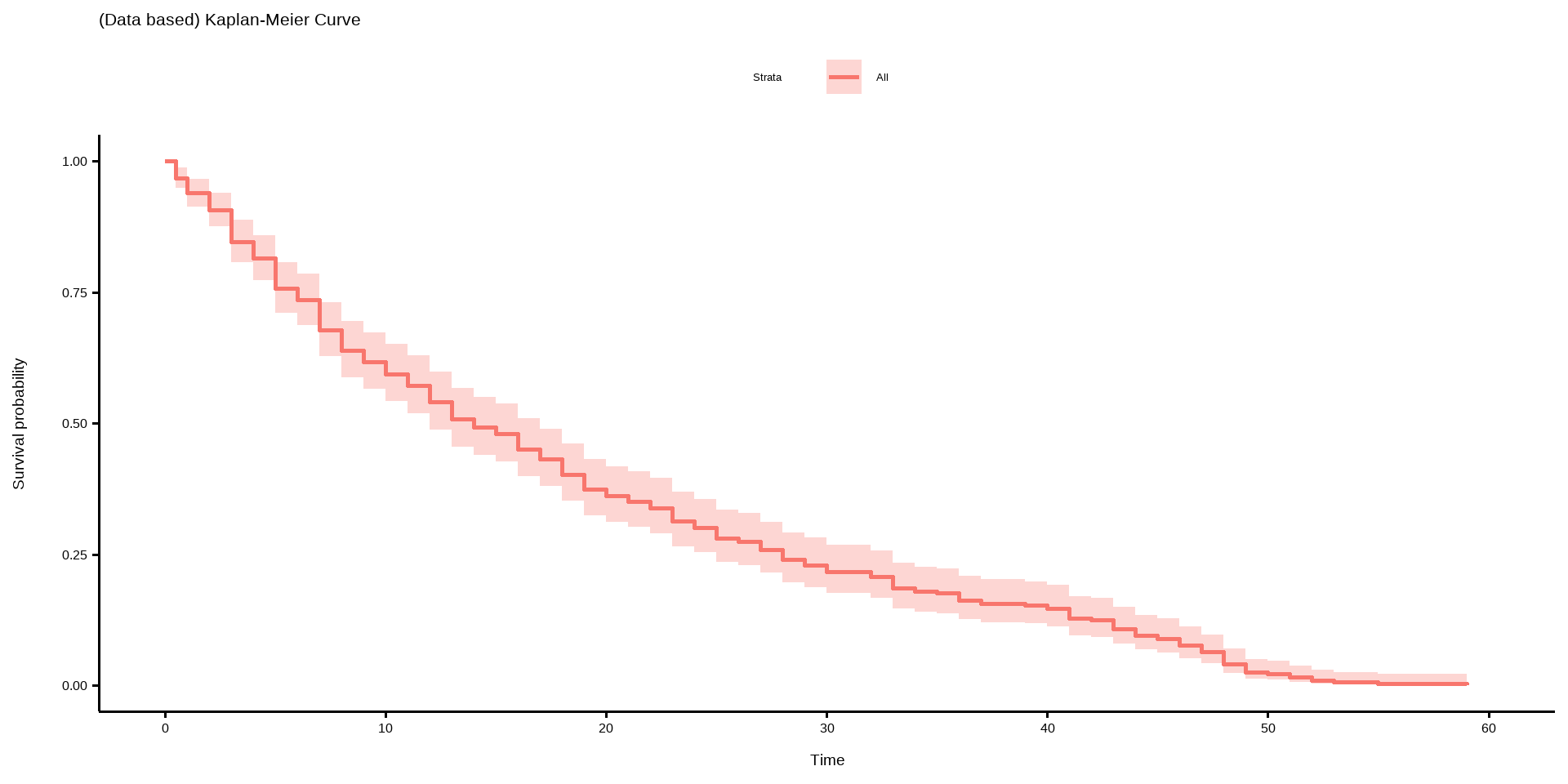
3.10 Kaplan-Meier Curve¹

Kaplan-Meier curve shows what the probability of an event (for example, survival) is at a certain time interval.

1. A.k.a, product limit estimator, often used in medical research

3.11 Estimation

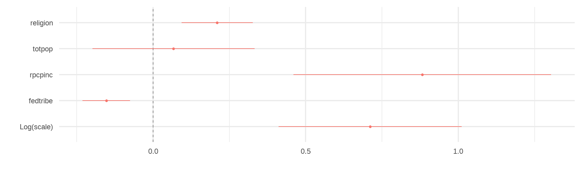
library(survival)

m_logit <-
  survreg(
    Surv(time = year, event = adopt_ig) ~ religion + totpop + rpcpinc + fedtribe,
    data = df_iga,
    dist = "logistic"
  )

dwplot(m_logit, vline = geom_vline(xintercept = 0, colour = "grey50", linetype = 2))

4 Duration Model

4.1 Duration: An Alternative

EH vs. Duration

Event history：事件发生的时间点

Duration：总体时间段

Duration Data

duration	opposition	polarization	Beilgium	Canada
3	-0.86792	11	1	0
7	-0.86792	11	1	0
20	-0.14103	11	1	0
6	-0.14103	11	0	1
17	-0.58065	6	0	1
7	-0.79592	3	0	1

4.2 Modeling the duration

• 选择
  • Parametric models
  • Semi-parametric models (e.g., cox)
• 选择本质：选定baseline hazard

最常见的四种参数模型

1. Exponential
2. Weibull
3. Log-normal
4. Gamma

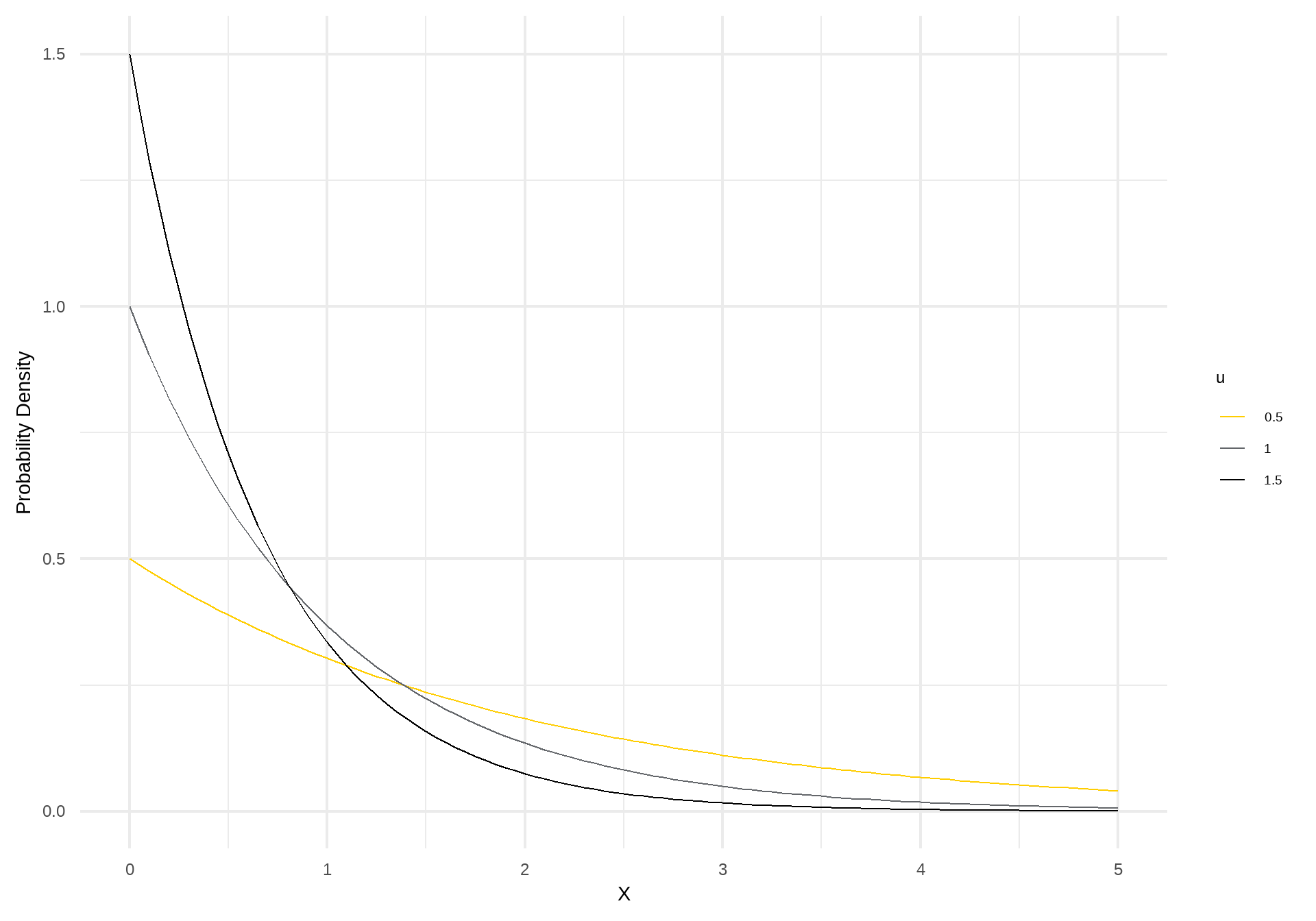
4.3 Exponential model

特点：Memoryless, hazard constant

\[ \begin{align} S(u) =& e^{-u} = f(u),\\ F(u) =& 1 - e^{-u},\\ h(u) =& 1 \end{align} \]

exponential: \(e^n\)

4.4 Weibull

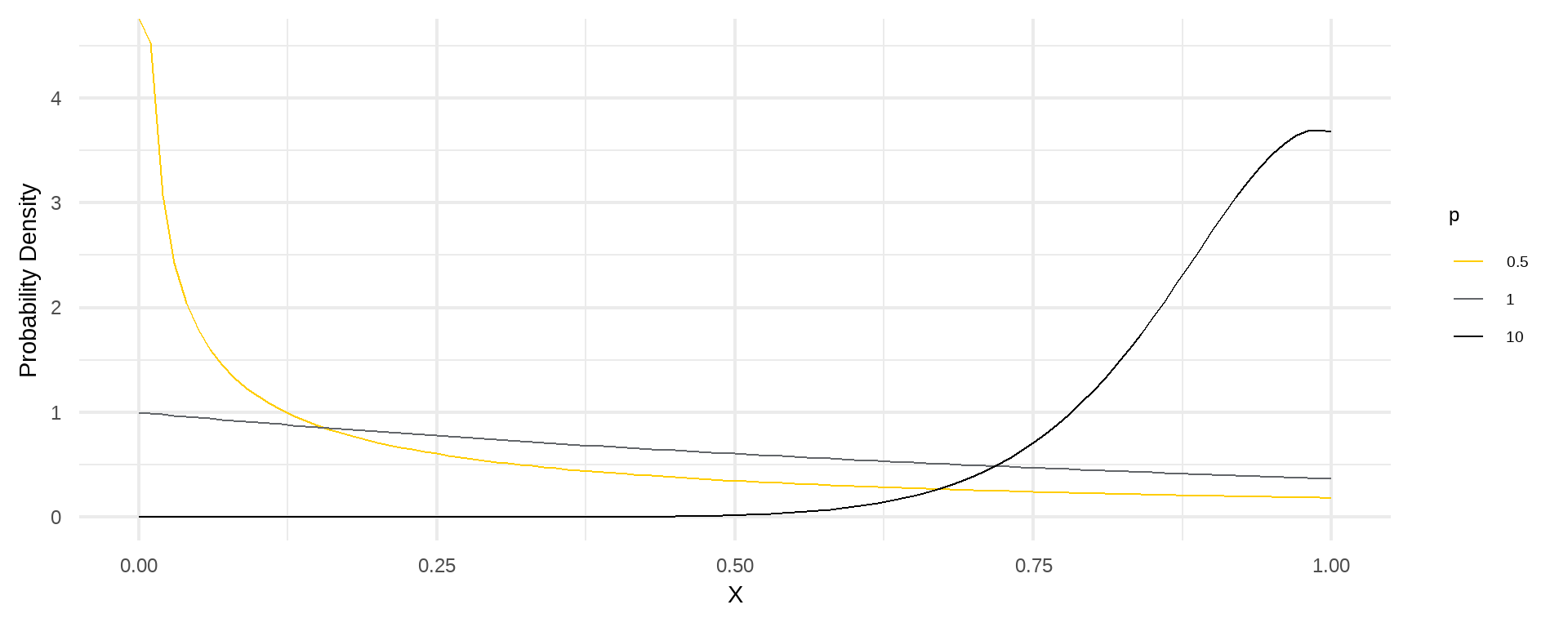
特点：用p调节baseline方向

p < 1, 单减
p = 1, = exponential
p > 1, 单增

\[ \begin{align} S(u)_{exp} =& e^{-u}\rightarrow S(u)_{weibull} = e^{-u^\color{red}{p}},\\ F(u) =& 1 - e^{-u^p}; f(u) = pu^{p - 1}e^{-u^p},\\ h(u) =& pu^{p - 1} \end{align} \]

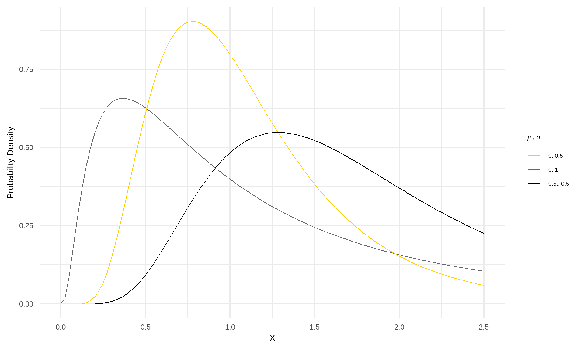
4.5 Log-normal

特点： 允许非单调hazard, \(ln(u_i)\sim N(\mu, \sigma^2).\)

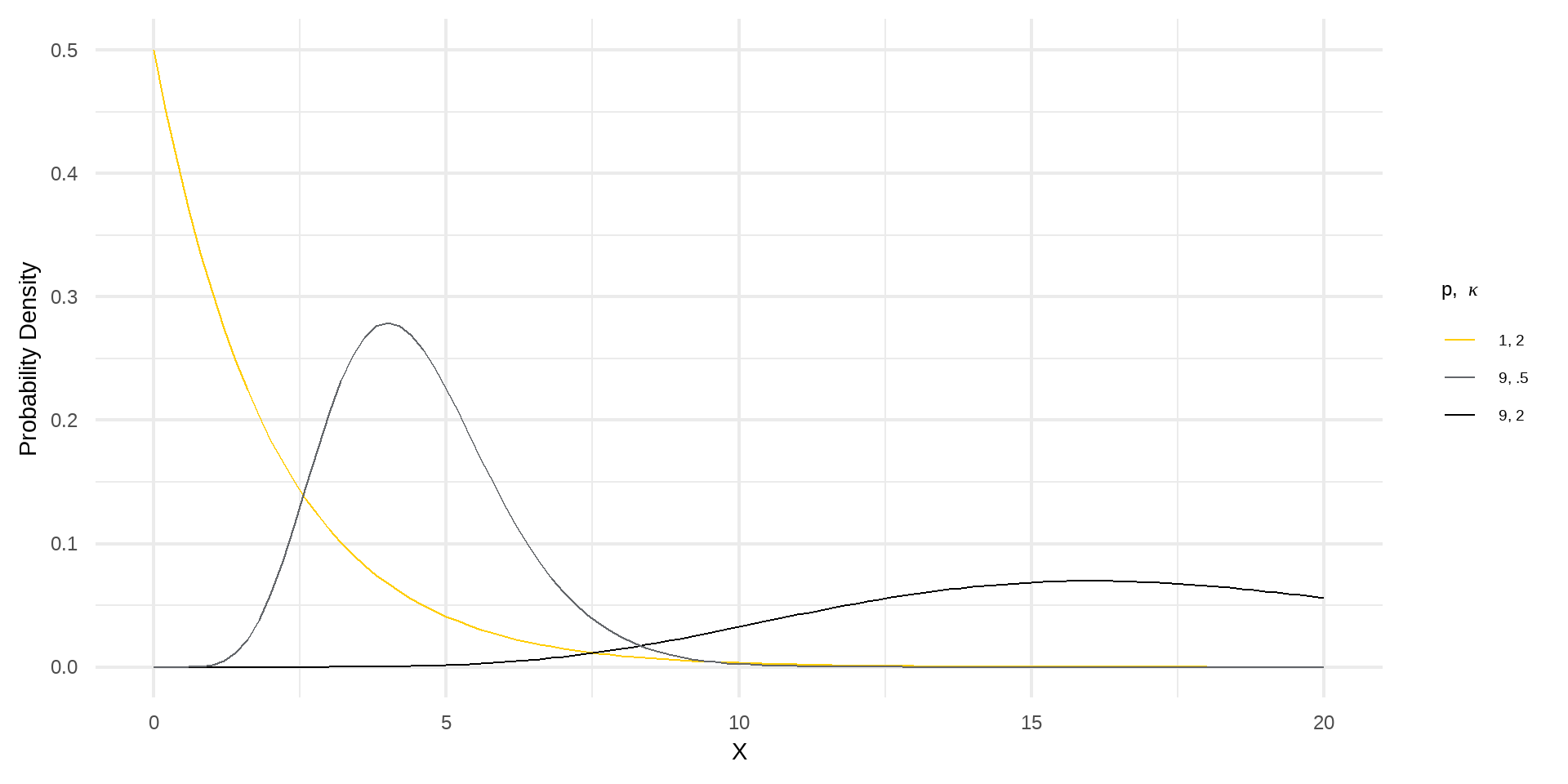
4.6 Gamma(Γ)

p: the scale parameter
κ: the shape parameter

\[ f(u) = pu^{p - 1}e^{-u^p}\rightarrow f(u) = \frac{pu^{p\color{red}{\kappa} - 1}e^{-u^p}}{\color{red}{\Gamma(\kappa)}}. \]

4.7 Bonus: Generalized Γ Distribution

\[f(u) = \frac{\color{orange}{p}u^{\color{orange}{p}\color{blue}{\kappa} - 1}e^{-u^\color{orange}{p}}}{\color{red}{\beta}^{\color{orange}{p}\color{blue}{\kappa}}\Gamma(\color{blue}{\kappa})}\]

β = 1 ⇒ Gamma;

κ = 0 ⇒ log-normal;

κ = 1 ⇒ Weibull;

κ = p = 1 ⇒ Exponential.

\(\beta\): 能存活的时间。

Exponential，Weibull，Log-normal, Gamma 都是Generalized Gamma的特殊变形

Ref: http://reliawiki.org/index.php/The_Generalized_Gamma_Distribution

4.8 X改变的是什么

Expected value

• Exponential: \(E(Y_i|X_i) = \lambda_i^{-1} = exp(X_i\beta)\)
• Weibull: \(E(Y_i|X_i) = \Gamma(p)exp(X_i\beta)\)

Hazard ratio

\[ \begin{align} \frac{h(Y_i|X + 1)}{h(Y_i|X)} =& \frac{pexp[-(X_i + 1)\beta]^py_i^{p - 1}}{pexp(-X_i\beta)^py_i^{p - 1}}\\ =& exp(-\beta)^p = e^{\color{red}{-\beta p}} \end{align} \]

-βp: proportional hazard metric;

β: accumulative failure time metric.

4.9 解释Harzard

\(Y_i = e^{X_i\beta}u_i\Rightarrow u_i = \frac{Y_i}{e^{X_i\beta}} = Y_ie^{-X_i\beta}\).

令\(\lambda\equiv e^{-X_i\beta}\), 那么，对于exponential

\[ \begin{align} u_i =& Y_i\lambda_i \\ F(Y_i|X) =& 1 - e^{-Y_i\lambda_i}\\ f(Y_i|X) =& \lambda_ie^{-Y_i\lambda_i}\\ h(Y_i|X) =& \lambda_i = e^{-Y_i\lambda_i} \end{align} \]

同理，对于Weibull, \(h(Y_i|X) = p\lambda^pY^{p - 1}.\)

4.10 Semi-parametric model

Cox model：不对Baseline hazard形状做假设

令\(\lambda\equiv e^{-X_i\beta}\)，

\[ \begin{align} h(t|x) =& \overbrace{h_0(t)}^{Non-parametric}\lambda_i^p,\\ P(1fails@t_1|someone\ f@t_1) =& \frac{h_0(t_1)\lambda_i^p}{\sum^n_{i = 1}h_0(t_1)\lambda_i^p},\\ P(2fails@t_2|someone\ f@t_2) =& \frac{h_0(t_2)\lambda_i^p}{\sum^n_{i = 2}h_0(t_1)\lambda_i^p} \end{align} \]

由于不是完全parametric，所以多只进行局部检验，因此不常在早期政治科学研究中出现。

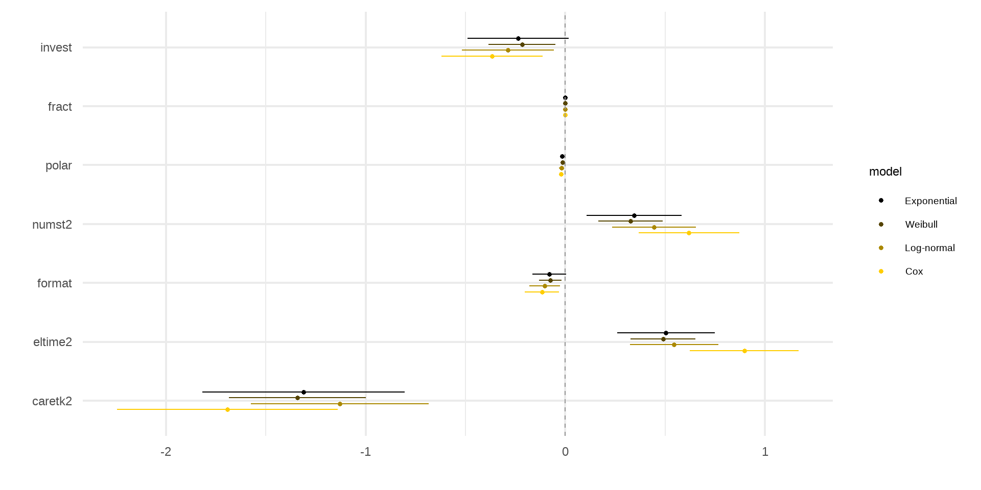
4.11 应用实例

Random tree for duration: https://rviews.rstudio.com/2017/09/25/survival-analysis-with-r/

4.12 Want to be an Expert Expert

Operation

Survival Analysis with R

Survival Task View

4.13 Take-Home Points

• 持续时间分析概念
  • 事件发生/结束的“点”与“线”
  • 大数据最基础数据
• 持续时间分析模型
  • Count
  • Discrete: logistic
  • Duration: exponetional, weibull, log-normal, cox
• 模型选择：Count, binary, duration—de-information

• 特殊情况
  • Duration dependency
  • Censored data
  • Time Varying Covariates
  • Repeated Failure
  • Competing Risk
  • Ties
  • Split Population
  • Non-proportional Hazard
  • Rare events

5 附录：特殊情况

5.1 持续时间分析会作什么妖

• Duration dependency (e.g., life-stage effects)
• Censored data (yeah, you can’t see it)
• Time Varying Covariates （Cox does not allow TVC)
• Repeated Failure (屡战屡败/屡败屡战)
• Competing Risk (What if the events are not indepdent)
• Ties (Tie in competition)
• Split Population (不败 vs. 不败yet)
• Non-proportional Hazard (每个观测点的basedline hazard function都一样吗？)
• Rare events (e.g., wars, human traffic, being an genius)
  ……

5.2 Duration Dependency

Baseline hazard随时间改变

解决方法:

• Fixed effect
• Smooth function: \(t, t^2, t^3\)(“nearly identical substantively [with spline]”).¹

• Spline

1. Carter, David B., and Curtis S. Signorino. 2010. “Back to the Future: Modeling Time Dependence in Binary Data.” Political Analysis 18(3): 271–92.

5.3 Rare Event

对于小概率事件（< 5%）→ 使用logit会高估Pr(Y = 1)。

解决方法：¹

假定没有其他更好sample

1. Prior correction: 加入基于其他研究或研究者认知的关于总体分布的趋势估计。
   • 注意：如果模型有误的话，结果也不会稳健。
2. Post-estimation weighting: \[P(Y_i = 1) \approx \tilde{\pi_i} + C_i,\] \(C_i\)输入某些总体分布信息。

1. King, Gary, and Langche Zeng. 2001. “Logistic Regression in Rare Events Data.” Political analysis 9(2): 137–63.

5.4 Last but not the least

三种将时间纳入事件的方式 (Count, binary, duration)，选哪个？

	Pros	Cons
Count	Aggregative, prevent measurement error	Lose the ability to record any identified variations over time and the time series
Duration	Record the time and changing moment and sequences	Lose the precision of when within each time unit an event occurs
Binary	Most disaggregate	Lose when the change happens in a time line

• 三种方法都是对同一现象的反映¹
• 三种models实际解释可能不一样，因为都是对现实的de-information

https://rviews.rstudio.com/2022/09/06/deep-survival/

1. Carstensen, Bendix. 2012. “Who Needs the Cox Model Anyway.” Stat Med 31: 1074–88, demonstrating the equivalence of the Cox model to a particular Poisson regression.

5.5 (Right) Censor

Censored point为c, 则：

\[ L = \prod^{n}_{i=1}f(y_i|x_i)^{1 - c}S(y^c|X_i)^c, \] where

\[c = \begin{cases} 1 & \text{if } y_i\geq y_c, \\ 0 & \text{if } y_i< y_c. \end{cases} \]

当censored部分扩大，模型的efficiency会降低。

如将selection effect也考虑进去的时候，需要modeling selection process¹

1. Boehmke, Frederick J., Daniel S. Morey, and Megan Shannon. 2006. “Selection Bias and Continuous-Time Duration Models: Consequences and a Proposed Solution.” American Journal of Political Science 50(1): 192–207.

5.6 Time Varying Covariates (TVC)

Assumption (Cox): Covariates do not vary over time.

Discrete model: Combine in the logit

Parametric: Conditional likelihood function (CTD: Continuous Time Duration)

\[ \begin{align} P(y_i>1|X_1(1)) =& \frac{P(y_i>2, y_i>1|X_1(2))}{P(y_i>1|X_1(2))}\\ =& S(1|X_1(1))p(y_i>2|y_i>1, X_1(2))\\ =& \frac{S(2|X_1(2))}{S(1|X_1(2))} \end{align} \]

Cox: put the value of that time moment, \(X_i(t)\), at failure time t in continuing the partial likelihood.

Partial likelihood:

\[\begin{align} L_p = \prod^K_{i = 1}[\frac{e^{X_i}\beta}{\sum_{j\in R(t_i)}e^{X_i\beta}}]^{\sigma_i} \end{align}\]

Assumption: intervals between successive duration time does not help to explain the relationship between covariates and hazard.

5.7 Repeated Failure

Type：

1. Total: 每次都重新开始
2. Gap: 从特定时间点开始计算
3. Counting: 每个观测点都在同一时间范畴，但允许晚进和censor

⇒ Risk set:

• Unrestricted: 在所有failure事件中，所有观测点无论之前经历过多少次failure都会继续在risk set中
• Semi-restricted: 在第K次failure事件中，risk set中只包含经历过k-1次或少于k-1次事件的观测点
• Restricted: 在第K次failure事件中，risk set中只包含经历过k-1次事件的观测点

5.8 估计方法

5.9 Competing Risk

两种方法：

• 假定竞争事件独立，进而分别建模——将竞争性视为censored
• 假定竞争事件非独立，引入shared frailties:

\[ \begin{align} h(y_1) =& h_0(y)exp(X\beta + v_1)\\ h(y_2) =& h_0(y)exp(X\beta + v_2) \end{align} \]

用\((v_1, v_2)\) jointed distributed 来纳入非独立性。

5.10 Tie

• Evenly divide λ in the nominators of two tied events.
• The most popular methods: Efron, Preslow.

5.11 Split Population (Cure Models)

可能有两种意义:

1. Never fail
2. Right censored

解决方法：

对Cure进行建模，\(Z_i\): 1 (cured), 0 (not cured), 其pdf为 \(P(Z_i = 1)\) , 那么对于0来说其survial model为 \(S(y|x)P(Z = 0)\).

5.12 Non-proportional Hazard

每个观测点的basedline hazard function都一样吗？

检验:

1. Piecewise regression
2. Model with interaction
3. Schoenfeld residual plot

解法

\[ y_i = X\beta_1 + Xln(t)\beta_2 + ln(t)\beta_3. \]