潜变量分析（前沿）

计算政治学讲习班

胡悦

清华大学社会科学学院

0.1 概述

1. 潜变量分析基础（复习）
2. 群组加权平均（MRP）
3. 群组项目反应理论之道
4. 潜变量分析的维度选择

1 潜变量分析基础

1.1 解决的问题

Vaild [latent variable] measurement is the cornerstone of successful scientific inquiry (Carpini and Keeter 1993, 1203).

涵盖所有社科学科

• 抽象
• 复杂
• 综合

操作性挑战

1. 不可见(Unobservable)
2. 有效果(Consequential)
3. 多维度(Multidimensional)

(Stimson 1991)

兜里有多少钱，不可见，但维度单一，不宜用潜变量分析，更好的办法是翻兜

The latent variable per se can’t be directly measured. But its consequences in opinions and behaviors can be observed.

1.2 平均值为什么不行

指标问题（1~10）：

1. 您是否信任身边人？
2. 您在政府机关有没有亲戚？
3. 您的朋友是否和您的想法经常一致？

累加综合法(additive scales)

\[\tilde{X} = (X_1 + X_2 + X_3)/3.\]

潜在问题

1. 相同权重(equal weight)
2. 结果不稳(extreme value sensitivity)
3. 忽略极化(polarity ignoring)

如何做得更好？

1.3 潜变量分析常见方法

连续因子模型

1. 探索性因子分析(EFA)
2. 结构方程模型(SEM)

离散回应模型

• 项目反应理论(IRT)
  • 项目反应群组估计

待解之题

1. 如何计算一个更靠谱的平均值
2. 如何正确使用群组潜变量分析
3. 如何判断潜变量的维度

2 群组加权平均计算

2.1 平均值在群组层面的问题

\[Y_{kq} = \frac{\sum Y_{ikq}}{n}.\]

不妥之处？

1. 如果群组过小，其平均值的代表意义不大
2. 不同的指标对于潜在变量贡献不一样

↓

经过群组信息（地理、人口）加权的平均值

Multilevel Regression and Post-stratification (MRP, Gelman and Little 1997)

2.2 Get the mean right

\[ \theta_h = \frac{\sum_{j \in h} N_j \color{red}{\mu_j} }{\sum_{j \in h} n_j}, \]

N: 总体（来自普查）
n: 样本（来自sample）

1. 将总体（population）按群组（strata，如国家、地区）切分；
2. 估测对象为核心变量在每个群组中的平均值/比例， θ_h (h ∈ {1, H});
3. 已知各群组以人口变量j（如老年男性、青年女性等）划分，确定群组人口（N_j）或占总人口比；
4. 通过multilevel model进行估算各组总体平均值μ_j。

2.3 一个经济学🌰

数据：某年某市五区域2396家产业公司的财政信息
目标：估测每个区域的产业平均收入

公司规模和区域分布

	A	B	C	D	E
Big	30	13	1	16	23
Medium	180	121	111	187	138
Small	97	593	862	20	4

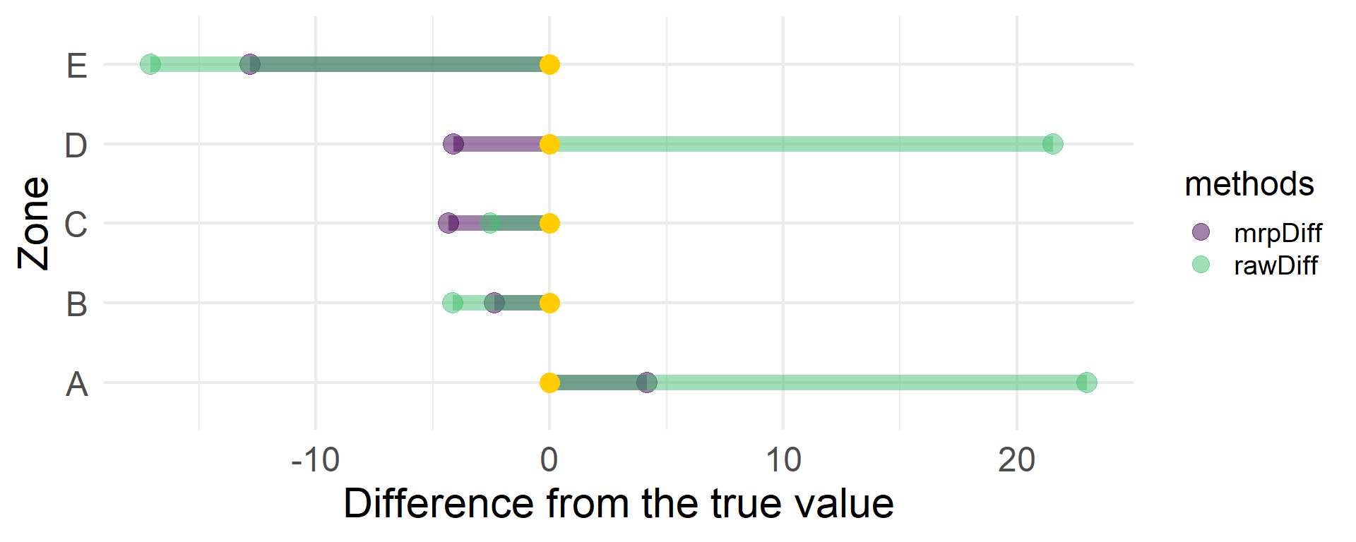
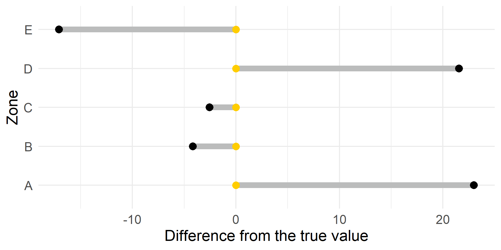
总体平均值（真值）

Zone	income
A	652.28
B	320.75
C	331.02
D	684.98
E	767.39

https://www.r-bloggers.com/gelmans-mrp-in-r-what-is-this-all-about/

2.4 样本

我们随机选取数据中1000个产业公司作为样本。 如果直接各组取平均值的话就会产生偏差：

2.5 计算

Step I: Mr \[ \begin{align} 收入 = \beta_{0z}& + \beta_{1Z=z}公司规模_{iz} + \epsilon_{iz}, \\ \beta_{0z}& = \gamma_{00} + \gamma_{01}区域_z + u_{0z}. \end{align} \]

Output: Post-strata means (\(\mu_z\))

	A	B	C	D	E
Big	1274.74	1148.58	1189.59	1238.51	1251.95
Medium	706.19	580.03	621.03	669.96	683.40
Small	372.95	246.79	287.79	336.72	350.16

Step II: P

       A        B        C        D        E 
656.4551 318.3753 326.6951 680.8675 754.5761 

2.6 矫正效果

MrP 没有解决的问题

• 答题难度的地区差异
• 题目的scale
• Measurement error

→ 群组IRT

3 群组IRT之“道”

3.1 群组IRT

Conquer the individual fallacy

Ecological fallacy (Simpson’s paradox)

再比如，民主、不平等、政治文化……

3.2 群组层级上的尝试 (Caughey and Warshaw 2015)

Dynamic Group-level IRT（DGIRT）

群组（Group-level）：¹

\(\eta_{ktq} = logit^{-1}(\frac{\color{red}{\bar{\theta}_{kt}}- \beta_q}{\sqrt{\alpha^2_q + \color{red}{(1.7\sigma_{kt})^2}}}),\)

\(\bar{\theta}_k\) 和 σ_kt 是潜在变量在组k时间t的均值和SD。

1. 在个体层面估测IRT；
2. 在估测IRT过程中加入群组级别变量；
3. 将时间变量融入IRT估测；
4. 用MrP给估测进行权重。

1.7: sd of probit is (π/3)^1/2 for logit, while Long 1997 found it is more close to 1.7 in actual estimations.

Mislevy, Robert J. 1983. “Item Response Models for Grouped Data.” Journal of Educational Statistics 8(4): 271–88.

η: eta

纳入时空 (Dynamic)

\[ \begin{align} \bar{\theta}_k\sim& N(\xi_t + \boldsymbol{x'_k\gamma}, \sigma^2_{\bar{\theta}}), \\ \xi_t \sim& N(\xi_{t-1}, \sigma^2_{\gamma}), \\ \gamma_{pt} \sim& N(\gamma_{p,t-1}, \delta_t + \boldsymbol{z'_p.\eta_t}, \sigma^2_{\gamma}) \end{align} \]

ξ_t: xi

x 为群组级变量

t-1, dynamic linear model

z’_p.η_t: geography-level attributes, η是coefficients

n^*_kqt基于MrP

效果：

• 囊括诸多因素
• 可以部分平衡样本代表性问题
• 强大，但复杂

Caughey & Warshaw称会跑几个星期

1. 个体：\(p_{iq} = logist^{-1}[\frac{\theta_i - {\beta_q}}{\alpha_q}].\)

3.3 简化版DGIRT (Claassen 2019)

\[ \begin{align} \eta_{ktq} = logit^{-1}&(\frac{\bar{\theta}'_{kt}- \beta_q}{\sqrt{\alpha^2_q + (1.7\sigma_{kt})^2}}).\\ \downarrow&\\ \eta_{ktq} = logit^{-1}&(\frac{\bar{\theta}'_{kt}- (\beta_q \color{red}{+ \delta_{kq}})}{\alpha_q}). \end{align} \]

δ_kq: 问题的difficulty随国家k变化。

1. 只作用于代表性样本和国家级别
   
2. 只对二分变量进行分析
3. 将国家作用从估测θ变为估测difficulty
   
4. 假定本地项目正态分布（忽略极化等现象😱）

3.4 纠偏版DGIRT (Solt 2020)

Dynamic Comparative Public Opinion

复杂程度：

Claasseen 2019 < DCPO < DGIRT

发表：

• APSR(Tai, Hu, and Solt 2024)
• BJPS(Woo, Goldberg, and Solt 2023)
• PSRM(Hu, Tai, and Solt 2024)
• SSQ(Woo et al. 2024)

……

3.5 效率比较

Bounded: 使用logit归为0-1

3.6 新方法面临新挑战

Source: urbanlogiq.com

劣质源数据

+

数据收集过程的难复刻性

+

难以追踪的人为操作

• The conventional approach usually involves a notorious bulk of manual work on indicator identification, data merging, data scaling, and so on
• Manual wrangling make a full reproducibility of research pipeline more difficulty and undermine the transparency
• Heterogeneous sources increases the risk
  • older survey files stored in SPSS’s ASCII or portable formats often require extensive restructuring before they can be merged with new format of data.
• Unfortunately, documentation does not cure everything, esp. the influence of human discretion embedded in manual processing

3.7 顶刊数据的例子

Here we provide a vivid example from real-life research to show how different results the seemingly basic, well-described hand-entered steps can produce. We attempted to replicate the spreadsheets applied in prominent studies following the replication instructions of the publications but with a more automatic process (elaborated below). Points on the diagonal show agreement; points above indicate higher hand-entered values, while points below show lower hand-entered percentages compared to machine-collected data.

For about 85% of country-year-item observations, differences between percentages are negligible-less than half a percent-resulting in points near the plot’s diagonal. However, for the remaining cases, differences are significant and cannot be ignored. These discrepancies stem from decisions on categorization, processing numerators and denominators in ratio calculation, and whether counting respondents excluded from original surveys. Though errors introduced during such processes seems minor and may appear as random noise, they can lead to opposite conclusions (Hu, Tai, and Solt 2024). Such issues pose a major, yet underrecognized, challenge to data harmonization in political science.

3.8 数据和谐之道（A TAO of Data Harmonization）

目标

1. 使用尽可能多的数据
2. 最大限度消除人工错误
3. 数据结果稳健性和可复制性

1. To incorporate as much available data as possible to provide a base for comparable data and increase generality of the inferences;
2. To reduce the manual entry errors to improve the accuracy of the harmonized data and analytic data; and
3. To improve the reproducibility of data wrangling process for the sake of transparency.

方法

1. Team-based concept construct and data selection;
2. Data entry automation and fully diagnoses;
3. “Second-order” opening.

演示案例

硬数据: SWIID

软数据: DCPO

• SWIID is a long-running project that seeks to provide harmonized income inequality statistics for the broadest possible coverage of countries and years
• DCPO is both a method and a database, to address the lack of cross-national and longitudinal data on many topics

3.9 Step 1: Team-Based Construct Building and Data Selection

目标问题

• “手残”之现实
  • 即使经过二次查验，数据整合错误率仍超过1% (Barchard and Pace 2011)
  • 金融和民航界惨痛教训(Haegemans, Snoeck, and Lemahieu 2019)

解法: Team work

• 概念构建
• 数据选择
• 合理性校验

Source: Barchard and Pace (2011, fig. 2)

• SWIID:
  • Told RAs that the goal of the research, a list of sources mainly from national statistic bureaus for them to start, but we also told them that update statistics for some countries may come from academic papers, published documents, and other sources, and they are free to add them in while making sure a valid link of the new sources are also recorded.
  • how the data would use later is also important, as they could have a better sense of what data are analyticable and a forward perspective of how many situations would the later entry part need to take care. In the SWIID project, we told the RAs that the inequality statistics be recorded in four formats: Gini index in disposable (post-tax, post-transfer) income, Gini in market (pre-tax, pre-transfer) income, absolute redistribution (market-income inequality minus net-income inequality), or relative redistribution (market-income inequality minus net-income inequality, divided by market-income inequality).
  • Cross-check: with new RAs
• DCPO: clearly defining and agreeing upon the latent construct among team members
  • Done by researchers not RAs
  • Each team member is then assigned survey datasets from specific geographic regions and tasked with identifying potentially relevant items and potential dimensions based on both general theoretical guidance and region-specific knowledge.
  • Before data selection begins, team members undergo hands-on training on how the method work and what type of data and detail they need to collect, such as data format and weighting types, which provide a valuable help of later build the automative data preparation software.
  • the dural-entry section comes in: each team member reviews and re-codes the survey data originally handled by another member.
  • Disputed cases are flagged for group discussion.

3.10 Step 2: Automation & Diagnosis

目标问题: 手动输入错误和结果“靠谱性”

解法: 尽可能地自动化

• Programming + API

• DCPOTools, countrycode, tabulapdf

3.11 DCPO操作自动化

1. 收集survey数据，明确与感兴趣的变量相关的指标问题（手动）
2. 通过DCPOtools对数据进行预处理（半自动）
3. 通过DCPO进行数据分析（自动）
4. 通过shinystan诊断convergence（自动）

诊断什么和如何理解

• Bayesian inference方法：Markov Chain Monte Carlo (MCMC)
• 数据拟合“底线”：Convergence
• 当Chain的posterior停留在一个相对稳定的区域内(ergodic chain)
  • \(\lim_{n\to \infty}p^n(\theta_i, \theta_j) = \pi(\theta_j), \forall \theta_i, \theta_j.\)

3.12 Step 3: “Second-Order” Opening

目标问题: 社会科学研究仍不够透明

解法: Second-order opening, 不止步于分析，还有DGP

Quarto

Github

OSF

If researchers applied our suggestions of team-based construct building, systematic data selection, and automated data entry, the second-order opening becomes both feasible and efficient. Along with a clearly conceptualized theoretical framework, researchers can simply share their programming scripts for data downloading, formatting, and wrangling, ensuring that the full pipeline is documented and reproducible.

With developed scientific and technical publishing system, such as Quarto or R markdown, and version control platforms (e.g., Github) and open collaboration platforms (e.g., Open Science Framework, OSF), researchers can integrate the entire workflow—from raw data collection to final analysis—within a single, publicly trackable archive. We reached at this step for all the DCPO projects so far.

3.13 未尽之事业

Source: Hu et al. 2025a, Fig 1

Source: Kuocheng Liao

4 潜变量分析的维度选择

4.1 如何确定看不见的维度

A.k.a., 你怎么知道只有一个潜在变量？

• 大部分IRT模型假定只有一个潜在变量

但社会科学中往往不是如此

4.2 迹象 (Hu et al. 2025)

4.3 理论标准

Measurement Invariance (Putnick and Bornstein 2016)

• 度量恒定性 (Metric invariance): 潜在变量的“一单位变化”在所有群体中都代表相同的含义
  • 有度量恒定性，即可比较关系系数（如相关性、回归系数等），但不能直接比较平均值
• 截距不变性 (Scalar invariance): 当两个比较对象的真实潜在水平相同，他们在不同群体中给出的观测值平均值也应相同。
  • 须在度量恒定性基础上实现

一个🌰

1. 度量不变性 (Metric invariance)

• 定义：不同群体中，潜在变量与测量指标之间的关系强度（即因子载荷）相同。
• 含义：潜在变量的“一单位变化”在所有群体中都代表相同的含义。
• 举例：如果“幸福感”增加 1 单位，在甲国和乙国，人们对“我经常微笑和大笑”这道题的平均回答都会增加同样的幅度。

👉 有度量不变性时，可以比较不同群体间的相关性或回归系数，但不能直接比较幸福感的平均水平。

2. 截距不变性 (Scalar invariance)

• 定义：在度量不变性的基础上，不同群体的测量指标的截距（intercepts）也相同。
• 含义：当两个人的真实潜在水平相同，他们在不同群体中给出的观测分数（如问卷回答）平均值也应相同。
• 举例：甲国和乙国两个同样幸福的人，在问卷上都会给出相似的回答（不会因为文化差异，一个答“同意”而另一个答“中立”）。

👉 有截距不变性时，研究者就可以比较群体间的潜在均值差异，也就是说，可以合理地说“甲国比乙国更幸福”。

换句话说：

• 度量不变性 → 不同群体用的是同样的“刻度单位”。
• 截距不变性 → 不仅刻度相同，而且零点基准也一致。

4.4 一种（间接）验证方法：CFM

EFA: 数据指向

1. 实证观察（归纳）
   • 无法统计推断
2. 未知维度
   • 每个维度都产生影响
3. 多重指标
   • Loading大小之分
4. 无视测量偏差关联
5. Underidentified

CFA: 理论指向

1. 理论定义（演绎）
   • 专为统计推断
2. 明确维度
   • 维度-指标关系明确
3. 单一指标
   • Loading有无之分
4. 允许测量误差相关
5. 必须identifiable

4.5 CFA指标选择

1. 严格依据理论：原因效果指标
2. 每维度一指标，艺术>技术

🌰 人际信任: 相信他人不会伤害自己或违背约定.

指标：

1. 总体而言，您是认同多数人是值得信任的，还是防人之心不可无？
2. 您认为多数时候人们是乐于助人的还是自私自利的？
3. 如果有机会，您认为别人是会占您便宜，还是说会恪守约定、公平行事？

4.6 另一个🌰：运动员评价

裁判对滑雪运动员的评判

单侧: factor complexity = 1 （一个变量只贡献一个latent）
双侧: factor complexity > 1

4.7 定义公式

Important

\[ \begin{align} X^* =& \Phi\Lambda' + \epsilon; \\ X =& \Lambda X_\xi + \epsilon, \end{align} \]

X： 指标向量
ξ：潜在变量
Λ_X: X = f(ξ)系数(a.k.a., loading, path)
ε：偏误向量

Φ: 潜在变量的协方差矩阵
Θ_ε: 偏误的协方差矩阵

ξ: ksi
δ: delta
Φ: phi
Θ_σ: theta

在EFA中潜在变量在等号左边，观测变量在右边

4.8 估算

潜变量矩阵

\[ \Phi = \begin{bmatrix} \phi_{11} & & \\ 0 & \phi_{22} & \\ 0 & \phi_{23} & \phi_{33} \end{bmatrix} \]

φ23$: classical 和showy 裁判的相关性

测量矩阵

\[ \begin{bmatrix} x_1\\ x_2\\ x_3\\ x_4\\ x_5 \end{bmatrix} = \begin{bmatrix} 1 & 1 & 0\\ \lambda_{21} & 1 & 0\\ \lambda_{31} & 1 & 0\\ \lambda_{41} & 0 & 1\\ \lambda_{51} & 0 & 1 \end{bmatrix} \begin{bmatrix}\xi_1\\ \xi_2\\ \xi_3 \end{bmatrix} + \begin{bmatrix}\epsilon_1\\ \epsilon_2\\ \epsilon_3\\ \epsilon_4\\ \epsilon_5 \end{bmatrix} \]

偏误矩阵

diag Θ_σ = diag[var(ε₁) var(ε₂)…var(ε₅)]

4.9 Identification

a.k.a., 最多能连多少线？

Identified: 当Λ、Φ、Θ存在唯一解

Λ: \(X = f(\xi)\)系数 (a.k.a., loading)；
Φ: 潜在变量的协方差矩阵；
Θ: 偏误的协方差矩阵。

t rule:

t < q(q + 1)/2

t: 不可见
q：可见

Another way to calculate df.

为保证identifable进行的限制

1. Scaling
   • λ₁₁ = 1;
   • 将潜在变量方差设为1(Standardized metric)
2. 参数调整
   • 特定因子loading设为0；
   • 偏误的协方差设为0；
   • 偏误的方差设为0.

4.10 求解

\[\Sigma(\theta) = \Lambda_X\Phi\Lambda_X' + \Theta_\epsilon,\] Σ: 所有可见指标得协方差矩阵

寻找最优Σ

全信息估计 (Maximum likelihood)

• Generalized Least Squares
  
• Unweighted Least Squares

有限信息估计

• Two Stage Least Squares

4.11 常见问题

错误：待分析的矩阵不是正定的

• 数据或协方差矩阵中录入错误
• 缺失数据
• 完全共线性
• 异常值

错误：不恰当的解

• 录入错误
• 总体值接近变量边界，加之抽样波动
• 模型错误
• 因素指标观测量过小（<150左右）且只有2个指标
• “Unlucky”样本
• 异常值

错误：未收敛

• 录入错误
• Unidentifiable
• 模型不佳
• 起始值不佳
• 小样本（N<100）
• 每个因素只有2指标
• 异常值
• 观测变量量纲极大差异

Error: Matrix to be analyzed not positive definite

• Typo in data file or covariance matrix
• Pairwise deletion of missing data
• Perfect collinearity
• Outliers/influential cases

Error: Improper solutions

• Typo in program
• Population value near the borderline combined with sampling fluctuation
• Specification error
• Small samples (<150 or so) combined with 2 indicators per factor
• “unlucky” sample
• Outliers/influential cases

Error: Nonconvergence

• Typo in program, data file, or covariance matrix
• Underidentified model
• Poor model specification
• Bad starting values
• Small samples (N<100)
• Only 2 indicators per factor
• Outliers/influential cases
• Observed variables in very different scale

4.12 诊断方法

Overall: χ²，结果显著¹则说明整体模型可能有问题。

1. Because models are almost always incorrect, any otherwise reasonably fitting model can be rejected when sample size is sufficient
2. Also a poor fitting model could be accepted if there is insufficient power to detect misspecification.

Incremental Fit Indices：将模型与基线模型比较

1. Tucker-Lewis Index (TLI, ρ₂, Non-Normed Fit Index)
2. Comparative Fit Index (CFI)

基线模型：只保留可见变量的方差和协方差

1 理想情况
<.95 不可接受

CFI可以>1, 这种情况视为1

Absolute Fit Indices

1. Root Mean Square Error of Approximation (RMSEA)
2. Standardized Root Mean Square Residual (SRMR)

• 0 理想情况
• ≤ 0.05 不错
• 0.05 ~ 0.08 差强人意
• ≥ 0.1 不可接受

1. 然而，当N足够大时χ²通常显著。

4.13 🌰 Holzinger & Swineford 1939

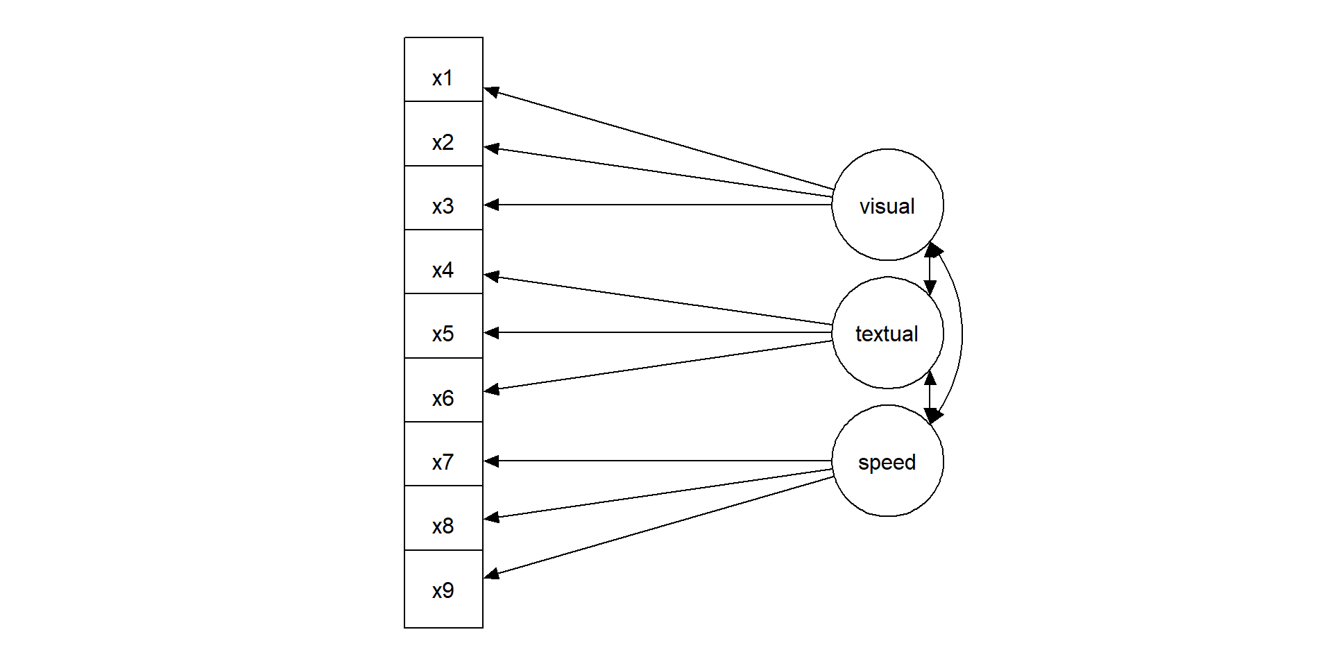
对初中生精神状况的调查： 视觉因素（x_1~3） + 阅读因素（x_4~6）+ （表达因素：x_7~9）

4.14 估测结果与诊断

lavaan 0.6-19 ended normally after 35 iterations

  Estimator                                         ML
  Optimization method                           NLMINB
  Number of model parameters                        21

  Number of observations                           301

Model Test User Model:
                                                      
  Test statistic                                85.306
  Degrees of freedom                                24
  P-value (Chi-square)                           0.000

Model Test Baseline Model:

  Test statistic                               918.852
  Degrees of freedom                                36
  P-value                                        0.000

User Model versus Baseline Model:

  Comparative Fit Index (CFI)                    0.931
  Tucker-Lewis Index (TLI)                       0.896

Loglikelihood and Information Criteria:

  Loglikelihood user model (H0)              -3737.745
  Loglikelihood unrestricted model (H1)      -3695.092
                                                      
  Akaike (AIC)                                7517.490
  Bayesian (BIC)                              7595.339
  Sample-size adjusted Bayesian (SABIC)       7528.739

Root Mean Square Error of Approximation:

  RMSEA                                          0.092
  90 Percent confidence interval - lower         0.071
  90 Percent confidence interval - upper         0.114
  P-value H_0: RMSEA <= 0.050                    0.001
  P-value H_0: RMSEA >= 0.080                    0.840

Standardized Root Mean Square Residual:

  SRMR                                           0.065

Parameter Estimates:

  Standard errors                             Standard
  Information                                 Expected
  Information saturated (h1) model          Structured

Latent Variables:
                   Estimate  Std.Err  z-value  P(>|z|)
  visual =~                                           
    x1                1.000                           
    x2                0.554    0.100    5.554    0.000
    x3                0.729    0.109    6.685    0.000
  textual =~                                          
    x4                1.000                           
    x5                1.113    0.065   17.014    0.000
    x6                0.926    0.055   16.703    0.000
  speed =~                                            
    x7                1.000                           
    x8                1.180    0.165    7.152    0.000
    x9                1.082    0.151    7.155    0.000

Covariances:
                   Estimate  Std.Err  z-value  P(>|z|)
  visual ~~                                           
    textual           0.408    0.074    5.552    0.000
    speed             0.262    0.056    4.660    0.000
  textual ~~                                          
    speed             0.173    0.049    3.518    0.000

Variances:
                   Estimate  Std.Err  z-value  P(>|z|)
   .x1                0.549    0.114    4.833    0.000
   .x2                1.134    0.102   11.146    0.000
   .x3                0.844    0.091    9.317    0.000
   .x4                0.371    0.048    7.779    0.000
   .x5                0.446    0.058    7.642    0.000
   .x6                0.356    0.043    8.277    0.000
   .x7                0.799    0.081    9.823    0.000
   .x8                0.488    0.074    6.573    0.000
   .x9                0.566    0.071    8.003    0.000
    visual            0.809    0.145    5.564    0.000
    textual           0.979    0.112    8.737    0.000
    speed             0.384    0.086    4.451    0.000

4.15 使用CFA确认/验证维度 (Jöreskog 1971)

Theory matters!

Using MGCFA to confirm dimensions

4.16 确认维度之后 (Berwick and Caughey 2025)

Multidimensional, multilevel IRT

• Strengths
  • Flexible: Single-country or cross-national datasets
  • Extensible: Overdispersion, differential item functioning, and predictors.
• Considerations
  • Computationally intensive (Bayesian estimation).
  • Needs bridging items for comparability across groups/time.

4.17 总结

• 平均值层次（MRP）
  • 计算具有总体意义的组别平均值
  • 需要组别分布
  • 局限
    • 问题差异
    • 答题差异
• 群组IRT（DGIRT，DCPO）
  • 计算群组层级可比度量
  • 操作
    • Team-work collection
    • Automation everything
    • Opening

• 分析维度判定
  • 验证性因子分析：检验潜在变量对于观察指标是否有影响
    • CFA诊断：χ², TLI/CFI，RMSEA/SRMR
  • CFA + IRT
    • MGCFA
    • MODGIRT

5 欢迎交流

  sammo3182

  yuehu@tsinghua.edu.cn

  https://sammo3182.github.io/

参考文献

Barchard, Kimberly A., and Larry A. Pace. 2011. “Preventing Human Error: The Impact of Data Entry Methods on Data Accuracy and Statistical Results.” Computers in Human Behavior 27 (5): 1834–39.

Berwick, Elissa, and Devin Caughey. 2025. “MODGIRT: Multidimensional Dynamic Scaling of Aggregate Survey Data.” Political Analysis, 1–16.

Carpini, Michael X. Delli, and Scott Keeter. 1993. “Measuring Political Knowledge: Putting First Things First.” American Journal of Political Science 37 (4): 1179–1206. https://doi.org/10.2307/2111549.

Caughey, Devin, and Christopher Warshaw. 2015. “Dynamic Estimation of Latent Opinion Using a Hierarchical Group-Level IRT Model.” Political Analysis 23 (2): 197–211. https://doi.org/10.1093/pan/mpu021.

Claassen, Christopher. 2019. “Estimating Smooth Country–Year Panels of Public Opinion.” Political Analysis 27 (1): 1–20.

Gelman, Andrew, and Thomas C. Little. 1997. “Poststratification into Many Categories Using Hierarchical Logistic Regression.” Survey Methods 23: 127–35.

Haegemans, Tom, Monique Snoeck, and Wilfried Lemahieu. 2019. “A Theoretical Framework to Improve the Quality of Manually Acquired Data.” Information & Management 56 (1): 1–14.

Hu, Yue, Yuehong Cassandra Tai, Kyein Ko, Byung-Deuk Woo, and Frederick Solt. 2025. “An Incomplete Recipe: One-Dimensional Latent Variables Do Not Capture the Full Flavor of Democratic Support.” Research & Politics 12 (2): 20531680251341857. https://doi.org/10.1177/20531680251341857.

Hu, Yue, Yuehong Cassandra Tai, and Frederick Solt. 2024. “Revisiting the Evidence on Thermostatic Response to Democratic Change: Degrees of Democratic Support or Researcher Degrees of Freedom?” Political Science Research and Methods, May, 1–7. https://doi.org/10.1017/psrm.2024.16.

Jöreskog, K. G. 1971. “Simultaneous Factor Analysis in Several Populations.” Psychometrika 36 (4): 409–26. https://doi.org/10.1007/BF02291366.

Putnick, Diane L., and Marc H. Bornstein. 2016. “Measurement Invariance Conventions and Reporting: The State of the Art and Future Directions for Psychological Research.” Developmental Review 41 (September): 71–90. https://doi.org/10.1016/j.dr.2016.06.004.

Solt, Frederick. 2020. “Modeling Dynamic Comparative Public Opinion.” SocArXiv.

Stimson, James A. 1991. Public Opinion in America: Moods, Cycles, and Swings. Transforming American Politics Series. Boulder: Westview Press.

Tai, Yuehong ‘Cassandra’, Yue Hu, and Frederick Solt. 2024. “Democracy, Public Support, and Measurement Uncertainty.” American Political Science Review 118 (1): 512–18. https://doi.org/10.1017/S0003055422000429.

Woo, Byung-Deuk, Lindsey A. Goldberg, and Frederick Solt. 2023. “Public Gender Egalitarianism: A Dataset of Dynamic Comparative Public Opinion Toward Egalitarian Gender Roles in the Public Sphere.” British Journal of Political Science 53 (2): 766–75. https://doi.org/10.1017/S0007123422000436.

Woo, Byung-Deuk, Hyein Ko, Yuehong Cassandra Tai, Yue Hu, and Frederick Solt. 2024. “Public Support for Gay Rights Across Countries and over Time.” Social Science Quarterly 106 (1): e13478. https://doi.org/10.1111/ssqu.13478.

6 附录：贝叶斯统计诊断

6.1 Convergence 特征

• 常返
  • 齐次/封闭：在第 \(m\) 步，如果此步的转移概率与 \(m\) 无关；对于状态 A、B，\(p(A, B) = 0\)
  • 不可约：如果从任意已达点/点集都可以到达其他任意已达点/点集；\(p(\theta_i, \theta_j) \neq 0, \ \forall \theta_i, \theta_j\)
• 平稳性：无自相关
• 非周期性：即使经过长时间，链的取值也不会出现相同的循环重复

• Reccurent

  • Homogeneous/Closed: At step m if the trasition probabilities at this step do not depend on m; for State A, B, p(A, B) = 0
  • Irreducible: If every reached point/point collection can be reached from every other reached point/point collection; p(θ_i, θ_j)≠ 0, ∀ θ_i, θ_j

• Stationary: no autocorrelation

• Aperodic: even with a long time there’s no identical cycle of chain values repeating

• Homogeneity: at step m the transition probability at this step do not depend on

• Ergodicity：遍历性

6.2 Converged时什么样：一个🌰

下雪啦天晴啦
下雪别忘穿棉袄
下雪啦天晴啦
天晴别忘戴草帽
带草帽~~~
—《心中的太阳》

今晴，明80%也晴；
今雪，明60%也雪。

		明天
		θ1	θ2
今天	θ1	0.8	0.2
	θ2	0.6	0.4

刘欢：《心中的太阳》, 《雪城》主题曲，1988年，倪萍主演

该曲采用再现三段体结构形式写成，外加一个高亢、悠扬的尾声。A段采用悠扬自由的散板节奏，具有思忖沉寂的意境。“大实话”式的歌词，饱含着对自然、社会、人生的不解、疑惑与诘问。B段开始转为充满活力的快板速度，歌词开始由诘问转变为对人间常态的肯定。A’段的旋律不变，只是节律变得富于急迫感、动力感，在这种动力的驱动下，继续开始诘问。高亢、悠扬的尾声，以反复咏唱的“啊太阳”结束，寓意作者对人间真理的无限向往与坚定追求

example of converged

起始点: [0.5 0.5]

\(S_1 = [0.5\; 0.5]\begin{bmatrix}0.8 & 0.2\\ 0.6 & 0.4 \end{bmatrix}=[0.7\; 0.3];\) \(S_2 = [0.7\; 0.3]\begin{bmatrix}0.8 & 0.2\\ 0.6 & 0.4 \end{bmatrix}=[0.74\; 0.26];\) \(S_3 = [0.74\; 0.26]\begin{bmatrix}0.8 & 0.2\\ 0.6 & 0.4 \end{bmatrix}=[0.748\; 0.252];\) \(S_4 = [0.748\; 0.252]\begin{bmatrix}0.8 & 0.2\\ 0.6 & 0.4 \end{bmatrix}=[0.749\; 0.250].\)

再往下算，会发现概率变化越来越小，趋于稳定（congverged）

6.3 检验Convergence

目前没有统计办法能够证明一个Markov Chain已经converged

1. 在给定时间内，无法保证Markov chain能够达到目标分布;
2. 无法预先确定一条Chain能够遍历目标分布的所有区域;
3. 只能诊断一条Chain是否未converged (诊断工具：Geweke’s G, Gelman-Rubin)

增加Convergence可能的方法

1. 足够的Burn-in rounds (诊断工具：Raftery-Lewis)
2. 尽可能排除autocorrelation（诊断工具：Heidelberger-Welch）

6.4 Geweke’s G

• 比较parameters在chain早期和晚期两个不重叠的窗口内的均值；
• 主要针对recurrence特征

\[G = \frac{\bar{\theta_1}- \bar{\theta_2}}{\sqrt{\frac{s_1}{n_1} + \frac{s_2}{n_2}}}.\]

A fancy difference of means

converge 则显示不显著差异，增加burn-in

6.5 Gelman & Rubin 1992

\[\hat{R}= \sqrt{\frac{\hat{var(\theta)}}{W}}\]

1. 跑多条chains（5~10），每条长2n
2. 对每一个感兴趣的parameter计算
   1. Within chain variance(W)
   2. Between chain variance(B)
3. 计算总体variance： var(θ) = (1 - 1/n)W + (1/n)B
4. 计算Scale reduction (亦称shrink factor)

Tip

• R趋近于1表示chains operating on same distribution
  • < 1.1或1.2是可以接受的

6.6 Burn-In

• 给与足够的burning in以到达目标分布
• “炸毛的毛毛虫”（Fuzzy Caterpillar）

6.7 检验Burn-in是否足够：Raftery & Lewis (1991, 1996)

• 分别评价每一个Chain的每一个变量
  1. 根据Chain间的相关性，并据此提供一个迭代数（iteration number）
  2. 检验autocorrelation inflation
• 输出
  • Burn-in：一位数或两位数为佳
  • Total：建议的burn-in数，未考虑cross-chain，因此真正burnin要乘上chain数
  • Dependence Factor

6.8 Autocorrelation

特征：

1. Chain间高相关性
2. 单一parameter高相关性

1. Chain间高相关性：Slow convergence
2. 单一parameter的高相关：Individual nonconvergence

Autocorrelated

Not autocorrelated

6.9 Heidelberger and Welch

用于检验Stationarity

1. 确定一个迭代数N, 以及准确性（ε）和显著性数准(α)
2. 运行整个chain
3. 施用Cramér-von Mises Test，Null: Chain是stationary
4. 如检验未通过则依次略去10%、20%,乃至50%的迭代，再次检测；
5. 如结果表示部分数据不是stationary，则对该部分数据进行halfwidth检验
6. 如果halfwidth ratio < ε, 则通过检验

6.10 Thinning

Thinning 并不会提高Chain的运算速度、帮助convergence或增强估测质量

• 每个Chain记录多少samples
  • Chain将仅记录第k个值，越高丢失的信息越多
  • k通常取值：4，5，10
• 仅用于降低autocorrelation

何时调Thin

1. 迭代中autocorrelation太高
2. Chain的convergence太低
3. 并行运算
4. 模型维度过高

7 附录：结构方程模型

7.1 什么是结构方程模型

• Structural equation model (SEM)
  
• LISREL (Linear Structural ReLationships) models
  
• Covariance structure models
  
• Latent variable models
  
• Structural equations with latent variables

• Confirmative factor analysis
  
• Multiple regression
  
• Multivariate regression
  
• ANOVA
  
• General linear model
  
• Path analysis
  
• Recursive models
  
• Dichotomous and ordered probit
  
• Seemingly unrelated regressions
  
• Simultaneous models
  
• Latent growth curve models
  ……

7.2 SEM (in terms of CFA)

结构

• 观察变量： X + Y
• 模型建构：
  1. Latent variable model
  2. Measurement model (CFA)
  3. Relations among the errors
• 依然要求identification

估计：MLE

诊断

• Overall：χ²
• Incremental：
  • TLI & CLI
  • Incremental Fit Index(IFI, Δ²)
• Absolute:
  • RMSEA
  • BIC

除了CFA，SEM还能做什么

敬请注意：SEM结果仍表现相关关系。

处理Measurement errors；处理非线性变量(hint: GSEM)；纳入多层效应；处理缺失值

7.3 🌰 Bollen 1989

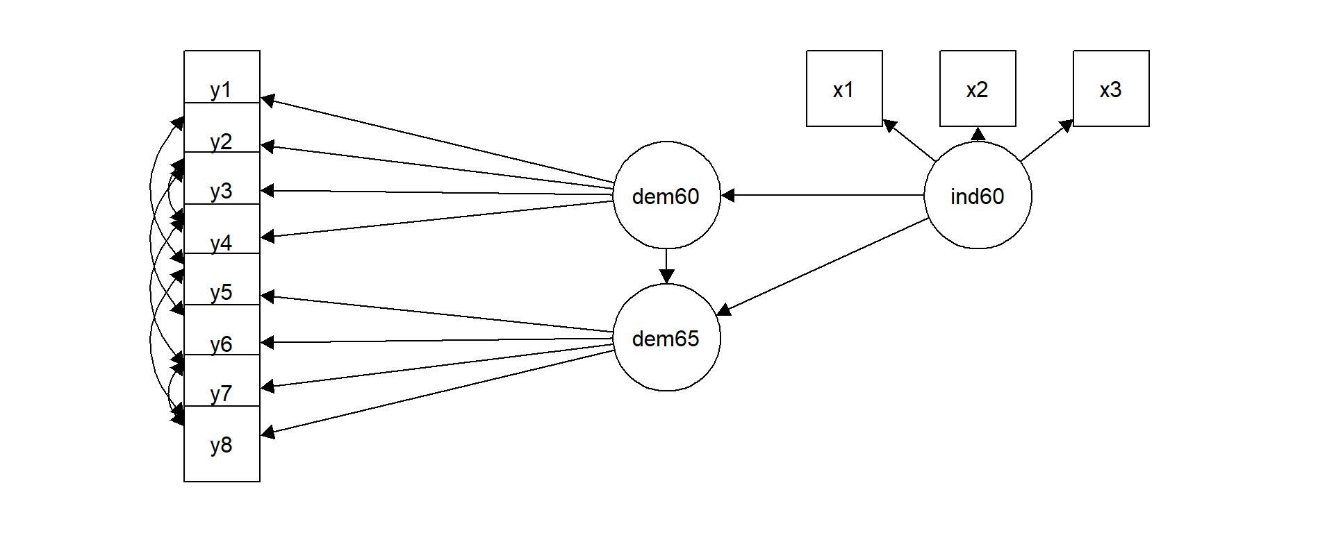
政治民主（1960，1965）与工业化

7.4 结果与诊断

lavaan 0.6-19 ended normally after 68 iterations

  Estimator                                         ML
  Optimization method                           NLMINB
  Number of model parameters                        31

  Number of observations                            75

Model Test User Model:
                                                      
  Test statistic                                38.125
  Degrees of freedom                                35
  P-value (Chi-square)                           0.329

Model Test Baseline Model:

  Test statistic                               730.654
  Degrees of freedom                                55
  P-value                                        0.000

User Model versus Baseline Model:

  Comparative Fit Index (CFI)                    0.995
  Tucker-Lewis Index (TLI)                       0.993

Loglikelihood and Information Criteria:

  Loglikelihood user model (H0)              -1547.791
  Loglikelihood unrestricted model (H1)      -1528.728
                                                      
  Akaike (AIC)                                3157.582
  Bayesian (BIC)                              3229.424
  Sample-size adjusted Bayesian (SABIC)       3131.720

Root Mean Square Error of Approximation:

  RMSEA                                          0.035
  90 Percent confidence interval - lower         0.000
  90 Percent confidence interval - upper         0.092
  P-value H_0: RMSEA <= 0.050                    0.611
  P-value H_0: RMSEA >= 0.080                    0.114

Standardized Root Mean Square Residual:

  SRMR                                           0.044

Parameter Estimates:

  Standard errors                             Standard
  Information                                 Expected
  Information saturated (h1) model          Structured

Latent Variables:
                   Estimate  Std.Err  z-value  P(>|z|)
  ind60 =~                                            
    x1                1.000                           
    x2                2.180    0.139   15.742    0.000
    x3                1.819    0.152   11.967    0.000
  dem60 =~                                            
    y1                1.000                           
    y2                1.257    0.182    6.889    0.000
    y3                1.058    0.151    6.987    0.000
    y4                1.265    0.145    8.722    0.000
  dem65 =~                                            
    y5                1.000                           
    y6                1.186    0.169    7.024    0.000
    y7                1.280    0.160    8.002    0.000
    y8                1.266    0.158    8.007    0.000

Regressions:
                   Estimate  Std.Err  z-value  P(>|z|)
  dem60 ~                                             
    ind60             1.483    0.399    3.715    0.000
  dem65 ~                                             
    ind60             0.572    0.221    2.586    0.010
    dem60             0.837    0.098    8.514    0.000

Covariances:
                   Estimate  Std.Err  z-value  P(>|z|)
 .y1 ~~                                               
   .y5                0.624    0.358    1.741    0.082
 .y2 ~~                                               
   .y4                1.313    0.702    1.871    0.061
   .y6                2.153    0.734    2.934    0.003
 .y3 ~~                                               
   .y7                0.795    0.608    1.308    0.191
 .y4 ~~                                               
   .y8                0.348    0.442    0.787    0.431
 .y6 ~~                                               
   .y8                1.356    0.568    2.386    0.017

Variances:
                   Estimate  Std.Err  z-value  P(>|z|)
   .x1                0.082    0.019    4.184    0.000
   .x2                0.120    0.070    1.718    0.086
   .x3                0.467    0.090    5.177    0.000
   .y1                1.891    0.444    4.256    0.000
   .y2                7.373    1.374    5.366    0.000
   .y3                5.067    0.952    5.324    0.000
   .y4                3.148    0.739    4.261    0.000
   .y5                2.351    0.480    4.895    0.000
   .y6                4.954    0.914    5.419    0.000
   .y7                3.431    0.713    4.814    0.000
   .y8                3.254    0.695    4.685    0.000
    ind60             0.448    0.087    5.173    0.000
   .dem60             3.956    0.921    4.295    0.000
   .dem65             0.172    0.215    0.803    0.422