潜变量分析（基础）

政务大数据应用与分析 (80700673)

胡悦

清华大学社会科学学院

提要

1. 概念与分析逻辑
   • 什么是潜变量
   • 怎么分析
2. 探索性因子分析
3. 验证性因子分析（与结构方程模型）*

操作语言

• R
  • psych
  • FactoMineR
  • laavan*

1 潜变量概念与分析逻辑

1.1 潜在变量 (Latent variables)

1.2 Why bother

Liberty leading the people

战狼II

同样行为背后的动机不同

• Liberty leading the people: the July Revolution of 1830 that toppled King Charles X，最终以查理十世退位导致波旁王朝灭亡、奥尔良公爵路易-菲利普继承王位告终，法国亦开始了奥尔良王朝的统治，但奥尔良王朝也不长命，亡于1848年的法国二月革命。

Vaild [latent variable] measurement is the cornerstone of successful scientific inquiry (Carpini and Keeter 1993, 1203).

涵盖所有社科学科

• 抽象
• 复杂
• 综合

操作性挑战

1. 不可见(Unobservable)
2. 多维度(Multidimensional)
3. 有效果(Consequential)

(Stimson 1991)

兜里有多少钱，不可见，但维度单一，不宜用潜变量分析，更好的办法是翻兜

The latent variable per se can’t be directly measured. But its consequences in opinions and behaviors can be observed.

1.3 分析逻辑

共因 → 结果

🌰 个体的社会资本（social capital）

指标问题（1~10）：

1. 您是否信任身边人？
2. 您在政府机关有没有亲戚？
3. 您的朋友是否和您的想法经常一致？

结果可见，共因不可见，以果推因

Three dimensions of social capital:

1. Trust
2. Norms
3. Networks

1.4 测量社会资本

指标问题（1~10）：

1. 您是否信任身边人？
2. 您在政府机关有没有亲戚？
3. 您的朋友是否和您的想法经常一致？

累加综合法(additive scales)

\[\tilde{X} = (X_1 + X_2 + X_3)/3.\]

潜在问题

1. 相同权重(equal weight)
2. 结果不稳(extreme value sensitivity)
3. 忽略极化(polarity ignoring)

如何做得更好？

1.5 因子分析基本模型

连续因子模型

1. 探索性因子分析(EFA)
2. 验证性因子分析(CFA)
3. 结构方程模型(SEM)

离散回应模型

• 项目反应理论(IRT)
  • 项目反应聚合估计

2 因子分析

2.1 基本原理

共因 → 结果

⇓

潜在变量 → 可见指标(indicators)

⇓

Minimum factors for the variances

determine the minimum number of hypothetical factors or components that account for the variance between variables.

2.2 操作挑战

• 目标: Fewer dimensons
• 决策:
  • 降到几维
    • 一维是是不是最优选择
  • 如何降维
    • 克服“累加法”缺陷

Exploratory FA

2.3 探索式因子分析

根本式 (Quinn 2004)

\[X^* = \Phi\Lambda' + \epsilon,\]

\(X^*\): 潜在变量
Φ: 指标选择
Λ: 单项贡献（a.k.a., factor loading）
ε 选择性误差

执行步骤

1. 个数选择
2. 因子提取
3. Rotation
4. 因子合成
5. 结果检验

2.4 🌰：人格测试

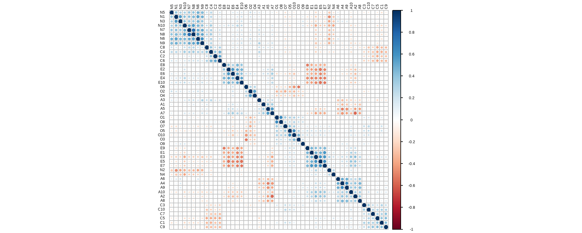
19,719 参与者, Big5 personality

2.5 实证数据

# A tibble: 19,719 × 57
    race   age engnat gender  hand source country    E1    E2    E3    E4    E5    E6
   <dbl> <dbl>  <dbl>  <dbl> <dbl>  <dbl> <chr>   <dbl> <dbl> <dbl> <dbl> <dbl> <dbl>
 1     3    53      1      1     1      1 US          4     2     5     2     5     1
 2    13    46      1      2     1      1 US          2     2     3     3     3     3
 3     1    14      2      2     1      1 PK          5     1     1     4     5     1
 4     3    19      2      2     1      1 RO          2     5     2     4     3     4
 5    11    25      2      2     1      2 US          3     1     3     3     3     1
 6    13    31      1      2     1      2 US          1     5     2     4     1     3
 7     5    20      1      2     1      5 US          5     1     5     1     5     1
 8     4    23      2      1     1      2 IN          4     3     5     3     5     1
 9     5    39      1      2     3      4 US          3     1     5     1     5     1
10     3    18      1      2     1      5 US          1     4     2     5     2     4
# ℹ 19,709 more rows
# ℹ 44 more variables: E7 <dbl>, E8 <dbl>, E9 <dbl>, E10 <dbl>, N1 <dbl>, N2 <dbl>,
#   N3 <dbl>, N4 <dbl>, N5 <dbl>, N6 <dbl>, N7 <dbl>, N8 <dbl>, N9 <dbl>, N10 <dbl>,
#   A1 <dbl>, A2 <dbl>, A3 <dbl>, A4 <dbl>, A5 <dbl>, A6 <dbl>, A7 <dbl>, A8 <dbl>,
#   A9 <dbl>, A10 <dbl>, C1 <dbl>, C2 <dbl>, C3 <dbl>, C4 <dbl>, C5 <dbl>, C6 <dbl>,
#   C7 <dbl>, C8 <dbl>, C9 <dbl>, C10 <dbl>, O1 <dbl>, O2 <dbl>, O3 <dbl>, O4 <dbl>,
#   O5 <dbl>, O6 <dbl>, O7 <dbl>, O8 <dbl>, O9 <dbl>, O10 <dbl>

经验开放性Openness, 尽责性Conscientiousness, 外向型Extraversion, 亲和性Agreeableness, 情绪不稳定型Neuroticism

https://quantdev.ssri.psu.edu/tutorials/intro-basic-exploratory-factor-analysis

• 降到几维
• 如何降维

2.6 维度选择

选择依据

概念关系 + 数据关系

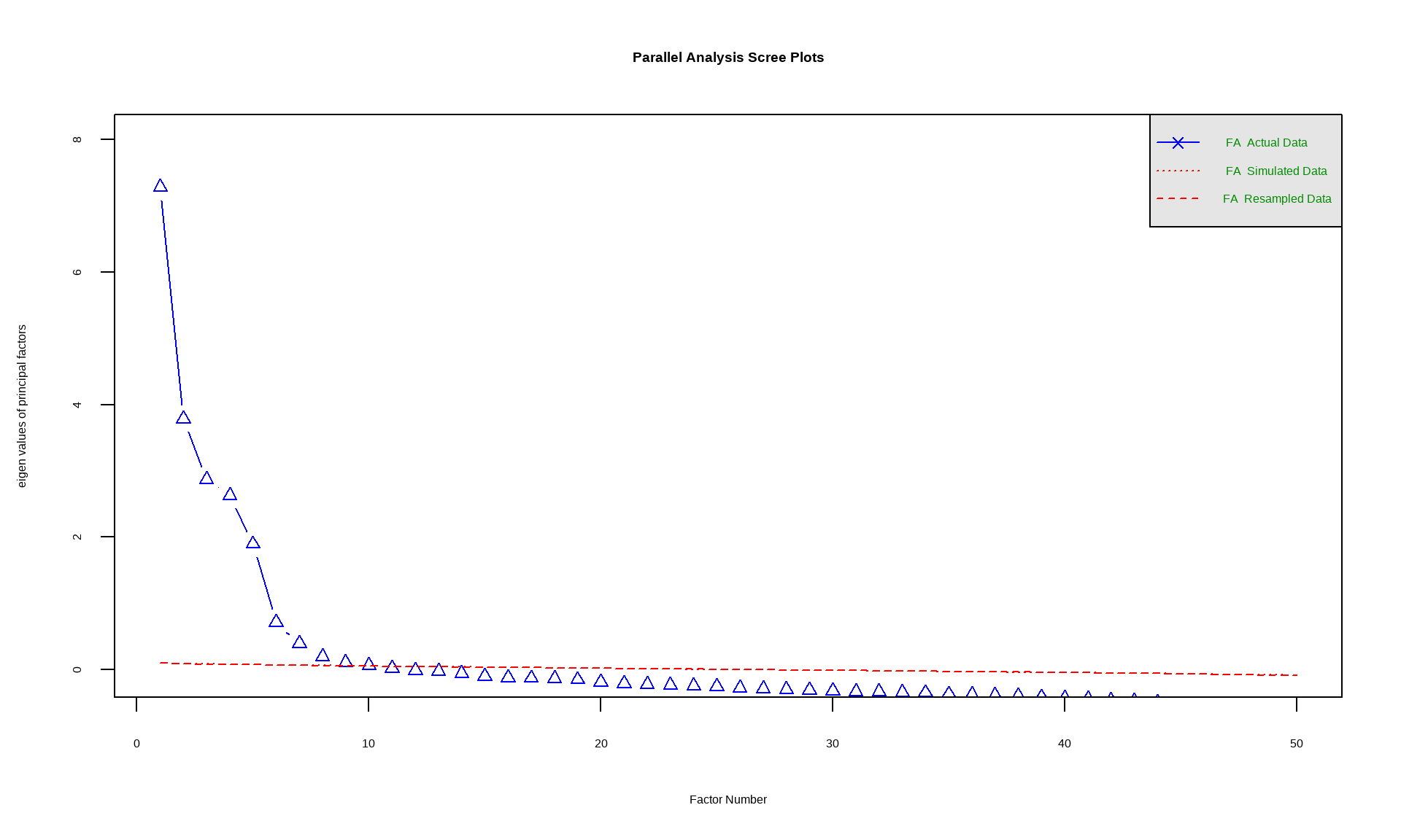
2.7 Horn’s Parallel Analysis

已知观测数据集O_m×n

1. 创建随机数据集R_m×n;
   
2. 相关矩阵_R → λ_R;
   
3. 相关矩阵_Ok → λ_Ok (k为因子数)
4. λ_Ok vs. λ_R

标准：

A. 如果λ_Ok < λ_R, 则 k B. Kaiser criterion: λ < 1 不可

2.8 因子提取(Factor Extraction)

• Minimum residual (OLS)
• Principal axes
• Alpha factoring
• Weighted least squares
• Minimum rank
• Maximum likelihood (ML, minimum χ² goodness of fit)

2.9 Rotation: 效果优化

Rotation:

A pattern of loadings where each item loads strongly on only one of the factors, and much more weakly on the other factors.

• Orthogonal: Varimax, quartimax, bentlerT, geominT, bifactor
  
• Oblique: Oblimin, quartimin, simplimax, bentlerQ, geominQ, biquartimin

Orthogonal(正交)

优选Oblique，允许factor间correlate

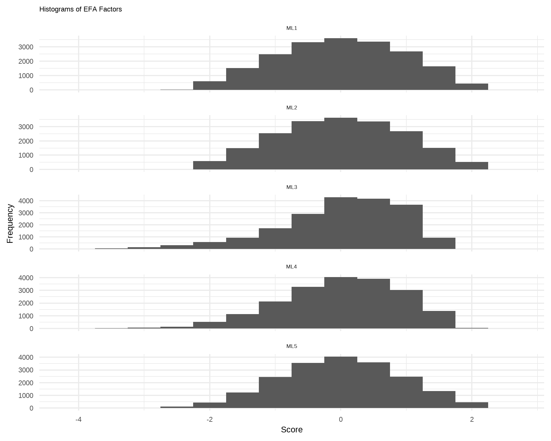
2.10 合成结果

ML + Oblimin

Loadings:
    ML1    ML2    ML3    ML5    ML4   
E1   0.691                            
E2  -0.697                            
E3   0.640                            
E4  -0.717                            
E5   0.732                            
E6  -0.547                            
E7   0.749                            
E8  -0.582                            
E9   0.623                            
E10 -0.662                            
N1          0.671                     
N2         -0.497                     
N3          0.593                     
N4                                    
N5          0.537                     
N6          0.746                     
N7          0.733                     
N8          0.760                     
N9          0.731                     
N10         0.576                     
A1                -0.432              
A2                 0.496              
A3                -0.404              
A4                 0.808              
A5                -0.652              
A6                 0.615              
A7                -0.582              
A8                 0.571              
A9                 0.713              
A10                0.334              
C1                        0.598       
C2                       -0.544       
C3                        0.395       
C4                       -0.531       
C5                        0.633       
C6                       -0.587       
C7                        0.555       
C8                       -0.454       
C9                        0.640       
C10                       0.466       
O1                               0.582
O2                              -0.537
O3                               0.538
O4                              -0.463
O5                               0.607
O6                              -0.502
O7                               0.492
O8                               0.552
O9                               0.346
O10                              0.679

                 ML1   ML2   ML3   ML5   ML4
SS loadings    4.912 4.409 3.601 3.174 3.163
Proportion Var 0.098 0.088 0.072 0.063 0.063
Cumulative Var 0.098 0.186 0.258 0.322 0.385

2.11 诊断

1. Sum of squared (SS) loading¹: 1
2. Communality/Uniqueness
3. Root means square of residuals(RMSR): 0.05
4. Tucker-Lewis Indes (TLI): 0.9
5. Reliability test (Crobach’s α)²

Factor analysis with Call: fa(r = ., nfactors = 5, rotate = "oblimin", fm = "ml")

Test of the hypothesis that 5 factors are sufficient.
The degrees of freedom for the model is 985  and the objective function was  3 
The number of observations was  19719  with Chi Square =  59071.56  with prob <  0 

The root mean square of the residuals (RMSA) is  0.03 
The df corrected root mean square of the residuals is  0.04 

Tucker Lewis Index of factoring reliability =  0.808
RMSEA index =  0.055  and the 10 % confidence intervals are  0.054 0.055
BIC =  49330.56
 With factor correlations of 
      ML1   ML2   ML3   ML5   ML4
ML1  1.00 -0.24  0.25  0.09  0.17
ML2 -0.24  1.00 -0.03 -0.24 -0.08
ML3  0.25 -0.03  1.00  0.14  0.07
ML5  0.09 -0.24  0.14  1.00  0.05
ML4  0.17 -0.08  0.07  0.05  1.00

• SS：Kaiser criterion: λ < 1 不可
• Communality: SS of all the factor loadings for a given variable
• Uniqueness: 1 - Communality
• RMSR < 0.05
• TLI > 0.9
• Crobach’s α: 计算因子分布的variables是不是内部一致，除非发表，不大必要

1. 特征值

2. 为每个因子分别计算

2.12 注意事项

• EFA是数据探索方法，不能用作统计推断
• EFA应用需满足以下假定:
  1. Linearity between the observed and latent
  2. Sufficient correlation between the observed and latent
  3. Homoscedasticity
  4. Multivariate normality among the observed
  5. No singularity among the observed
  6. Large N: 10 ~ 300
  7. Factorial Simplicity
• EFA不是唯一合理的降维方式
  • PCA
  • IRT

Red: bias; blue: efficiency

1. Linearity: EFA assumes a linear relationship between observed variables and underlying factors. This means that changes in the levels of factors are associated with proportional changes in the observed variables.

2. Multivariate Normality: Ideally, the observed variables should follow a multivariate normal distribution. While EFA can be performed on data that do not perfectly adhere to this assumption, deviations from multivariate normality can affect the robustness of the factor analysis, especially when estimating parameters and computing fit indices.

3. Adequate Sample Size: There is no strict rule for the minimum sample size in EFA, but a larger sample size can provide more reliable and stable factor solutions. A commonly cited guideline suggests having at least 5 to 10 observations per variable, though some scholars recommend a minimum of 300 cases as a more general benchmark.

4. No Perfect Multicollinearity or Singularity: While EFA aims to identify the underlying structure by exploring the correlations between variables, perfect multicollinearity (where one variable is a perfect linear combination of others) should be avoided. Similarly, singularity (where some variables are redundant) should be avoided, as these conditions can distort the analysis.

5. Sufficient Correlation: For a factor model to be meaningful, there must be some degree of correlation among the observed variables. If variables are completely uncorrelated, there would be no underlying factors to extract. The Kaiser-Meyer-Olkin (KMO) measure of sampling adequacy and Bartlett’s test of sphericity are commonly used to assess this assumption.

6. Homoscedasticity: The assumption of homoscedasticity (equal variances) among variables is also important for the generalizability of EFA results. Significant heteroscedasticity can lead to biased estimates of factor loadings and uniqueness.

7. Factorial Simplicity: This is more of a desired property than a strict assumption. Factorial simplicity implies that each variable should load strongly on one factor and have minimal loadings on other factors. This assumption facilitates the interpretability of factors.

Violations of these assumptions can lead to inaccurate factor solutions, misleading interpretations, and conclusions. It is therefore important to assess these assumptions before proceeding with EFA. In practice, some of these assumptions can be relaxed or addressed through data transformation, adopting robust estimation methods, or increasing the sample size.

2.13 Principal Component Analysis

根本式

\[C = w_iY_i,\]

C: Components， “因子”

Y: Measures

create one or more index variables (Components) from a larger set of measured variables (Y)

2.14 PCA vs. EFA

结果或近似，逻辑大不同

PCA: measurement to index

write all variables in terms of a smaller set of features which allows for a maximum amount of variance to be retained in the data.

EFA: indices to measurement (of a latent variable)

find a set of features which allow for understanding as much of the correlations between measured variables as possible. individually.

2.15 如何选择

• PCA最大程度保留可见变量信息，EFA旨在提取不可变量特征；
• 当Variable之间关系不那么紧密或受同一变量影响，PCA > EFA；
• 当估计潜在变量时，PCA可能夸大可见指标的影响

2.16 Bonus: 非连续变量PCA

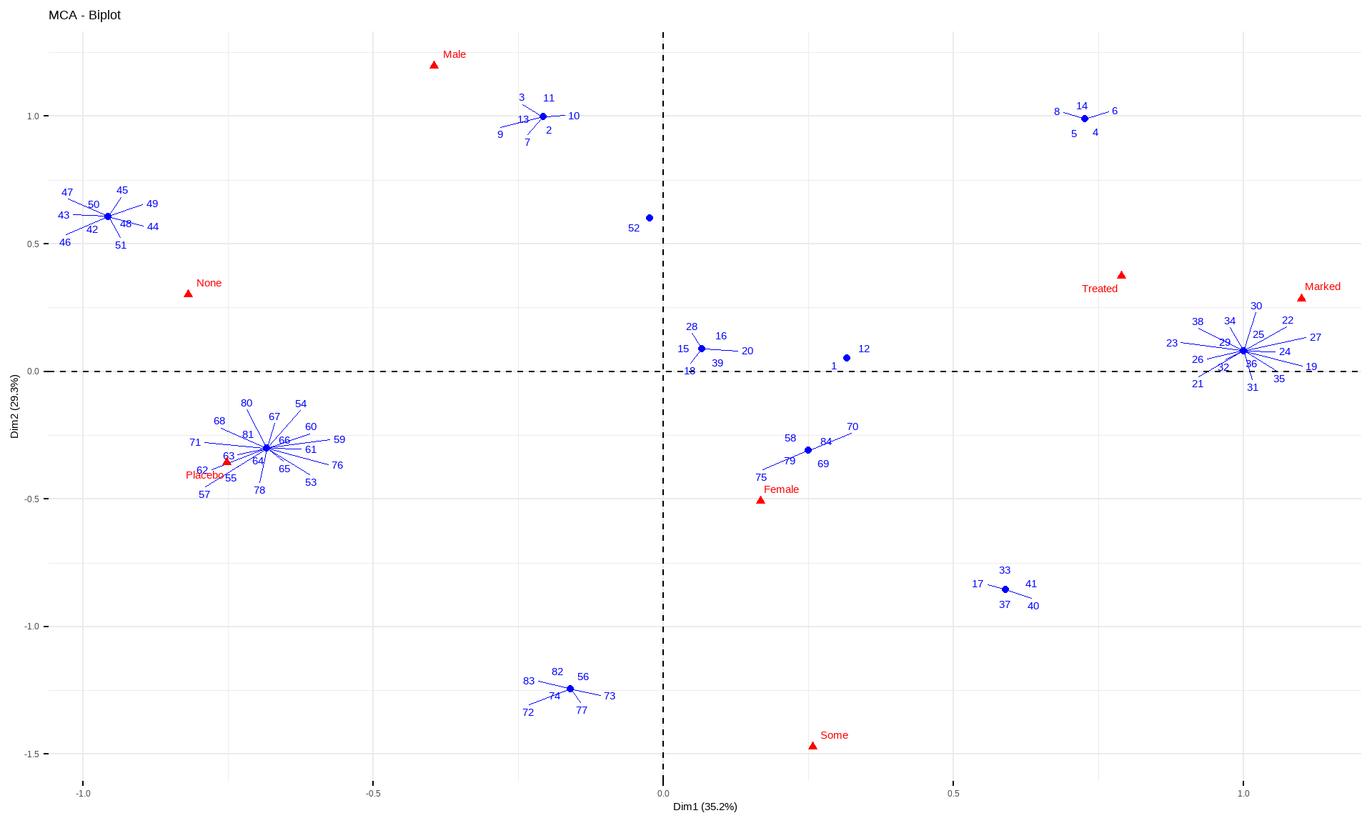
Multiple Correspondence Analysis (MCA, Husson, Le, and Pagès 2010)

2.17 Bonus: 混合变量的PCA

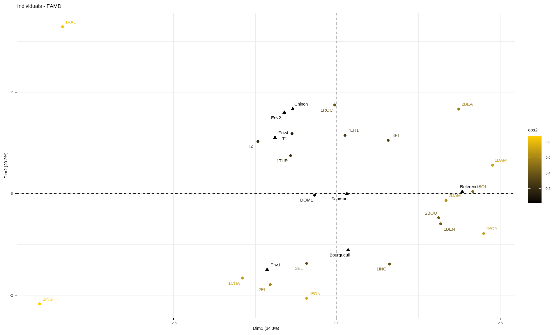
Factorial Analysis of Mixed Data (FAMD, Pagès 2004)

https://www.r-bloggers.com/2022/11/pca-for-categorical-variables-in-r/

• Factorial Analysis of Mixed Data
  • cos² statistic (cosine squared): how well a variable, individual, or category is represented by a given factor (dimension)

2.18 总结

• 潜在变量分析概述
  • 连续性因子分析
  • 离散型因子分析

• EFA
  • 探索性因子分析：通过loading找到潜在变量
  • EFA诊断：Kaiser’s criterion
  • EFA vs. PCA: 结果相似，逻辑不同

待解之题：观测变量与潜变量之间关系要是非线性的那该怎么办呢？

2.19 参考文献

Carpini, Michael X. Delli, and Scott Keeter. 1993. “Measuring Political Knowledge: Putting First Things First.” American Journal of Political Science 37 (4): 1179–1206. https://doi.org/10.2307/2111549.

Husson, Francois, Sebastien Le, and Jérôme Pagès. 2010. Exploratory Multivariate Analysis by Example Using r. 1st edition. Boca Raton, Fla.: CRC Press.

Pagès, J. 2004. “Analyse factorielle de données mixtes.” Revue de Statistique Appliquée 52 (4): 93–111.

Quinn, Kevin M. 2004. “Bayesian Factor Analysis for Mixed Ordinal and Continuous Responses.” Political Analysis 12 (4): 338–53. https://doi.org/10.1093/pan/mph022.

Stimson, James A. 1991. Public Opinion in America: Moods, Cycles, and Swings. Transforming American Politics Series. Boulder: Westview Press.

3 附录：验证性因子分析

3.1 探索性 vs 验证性

EFA: 数据指向

1. 实证观察（归纳）
   • 无法统计推断
2. 未知维度
   • 每个维度都产生影响
3. 多重指标
   • Loading大小之分
4. 无视测量偏差关联
5. Underidentified

CFA: 理论指向

1. 理论定义（演绎）
   • 专为统计推断
2. 明确维度
   • 维度-指标关系明确
3. 单一指标
   • Loading有无之分
4. 允许测量误差相关
5. 必须identifiable

3.2 CFA指标选择

1. 严格依据理论：原因效果指标
2. 每维度一指标，艺术>技术

🌰 人际信任: 相信他人不会伤害自己或违背约定.

指标：

1. 总体而言，您是认同多数人是值得信任的，还是防人之心不可无？
2. 您认为多数时候人们是乐于助人的还是自私自利的？
3. 如果有机会，您认为别人是会占您便宜，还是说会恪守约定、公平行事？

3.3 另一个🌰：运动员评价

裁判对滑雪运动员的评判

单侧: factor complexity = 1 （一个变量只贡献一个latent）
双侧: factor complexity > 1

3.4 定义公式

Important

\[ \begin{align} X^* =& \Phi\Lambda' + \epsilon; \\ X =& \Lambda X_\xi + \epsilon, \end{align} \]

X： 指标向量
ξ：潜在变量
Λ_X: X = f(ξ)系数(a.k.a., loading, path)
ε：偏误向量

Φ: 潜在变量的协方差矩阵
Θ_ε: 偏误的协方差矩阵

ξ: ksi
δ: delta
Φ: phi
Θ_σ: theta

在EFA中潜在变量在等号左边，观测变量在右边

3.5 估算

潜变量矩阵

\[\Phi = \begin{bmatrix} \phi_{11} & & \\ 0 & \phi_{22} & \\ 0 & \phi_{23} & \phi_{33} \end{bmatrix}\]

φ23$: classical 和showy 裁判的相关性

测量矩阵

\[ \begin{bmatrix} x_1\\ x_2\\ x_3\\ x_4\\ x_5 \end{bmatrix} = \begin{bmatrix} 1 & 1 & 0\\ \lambda_{21} & 1 & 0\\ \lambda_{31} & 1 & 0\\ \lambda_{41} & 0 & 1\\ \lambda_{51} & 0 & 1 \end{bmatrix} \begin{bmatrix}\xi_1\\ \xi_2\\ \xi_3 \end{bmatrix} + \begin{bmatrix}\epsilon_1\\ \epsilon_2\\ \epsilon_3\\ \epsilon_4\\ \epsilon_5 \end{bmatrix} \]

偏误矩阵

diag Θ_σ = diag[var(ε₁) var(ε₂)…var(ε₅)]

3.6 Identification

a.k.a., 最多能连多少线？

Identified: 当Λ、Φ、Θ存在唯一解

Λ: \(X = f(\xi)\)系数 (a.k.a., loading)；
Φ: 潜在变量的协方差矩阵；
Θ: 偏误的协方差矩阵。

t rule:

t < q(q + 1)/2

t: 不可见
q：可见

Another way to calculate df.

为保证identifable进行的限制

1. Scaling
   • λ₁₁ = 1;
   • 将潜在变量方差设为1(Standardized metric)
2. 参数调整
   • 特定因子loading设为0；
   • 偏误的协方差设为0；
   • 偏误的方差设为0；

3.7 最优解

\[\Sigma(\theta) = \Lambda_X\Phi\Lambda_X' + \Theta_\epsilon,\] Σ: 所有可见指标得协方差矩阵

寻找最优Σ

全信息估计 (Maximum likelihood)

• Generalized Least Squares
  
• Unweighted Least Squares

有限信息估计

• Two Stage Least Squares

3.8 常见问题

错误：待分析的矩阵不是正定的

• 数据或协方差矩阵中录入错误
• 缺失数据
• 完全共线性
• 异常值

错误：不恰当的解

• 录入错误
• 总体值接近变量边界，加之抽样波动
• 模型错误
• 因素指标观测量过小（<150左右）且只有2个指标
• “Unlucky”样本
• 异常值

错误：未收敛

• 录入错误
• Unidentifiable
• 模型不佳
• 起始值不佳
• 小样本（N<100）
• 每个因素只有2指标
• 异常值
• 观测变量量纲极大差异

Error: Matrix to be analyzed not positive definite

• Typo in data file or covariance matrix
• Pairwise deletion of missing data
• Perfect collinearity
• Outliers/influential cases

Error: Improper solutions

• Typo in program
• Population value near the borderline combined with sampling fluctuation
• Specification error
• Small samples (<150 or so) combined with 2 indicators per factor
• “unlucky” sample
• Outliers/influential cases

Error: Nonconvergence

• Typo in program, data file, or covariance matrix
• Underidentified model
• Poor model specification
• Bad starting values
• Small samples (N<100)
• Only 2 indicators per factor
• Outliers/influential cases
• Observed variables in very different scale

3.9 诊断

Overall: χ²，结果显著则说明整体模型可能有问题。¹

1. Because models are almost always incorrect, any otherwise reasonably fitting model can be rejected when sample size is sufficient
2. Also a poor fitting model could be accepted if there is insufficient power to detect misspecification.

Incremental Fit Indices：将模型与基线模型比较

1. Tucker-Lewis Index (TLI, ρ₂, Non-Normed Fit Index)
2. Comparative Fit Index (CFI)

基线模型：只保留可见变量的方差和协方差

1 理想情况
<.95 不可接受

CFI可以>1, 这种情况视为1

Absolute Fit Indices

1. Root Mean Square Error of Approximation (RMSEA)
2. Standardized Root Mean Square Residual (SRMR)

• 0 理想情况
• ≤ 0.05 不错
• 0.05 ~ 0.08 差强人意
• ≥ 0.1 不可接受

1. 然而，当N足够大时χ²通常显著。

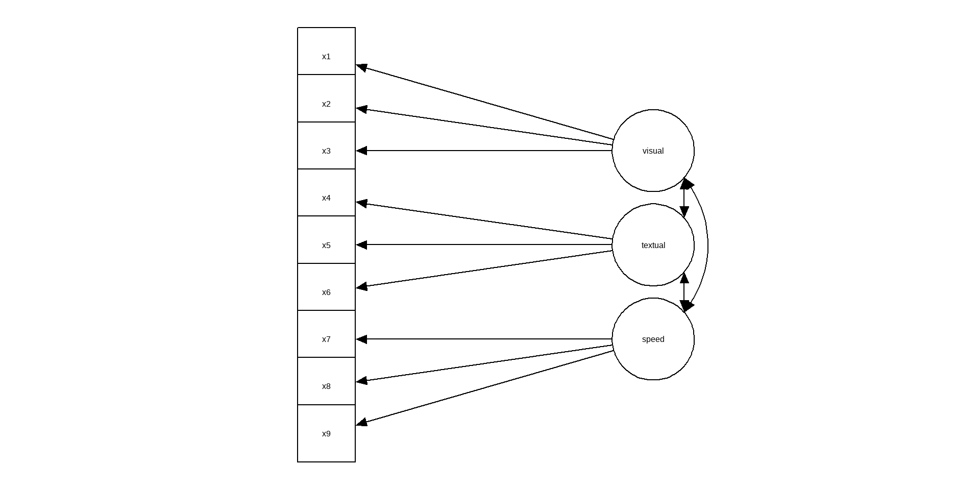
3.10 🌰 Holzinger & Swineford 1939

对初中生精神状况的调查： 视觉因素（x_1~3） + 阅读因素（x_4~6）+ （表达因素：x_7~9）

3.11 估测结果与诊断

lavaan 0.6-19 ended normally after 35 iterations

  Estimator                                         ML
  Optimization method                           NLMINB
  Number of model parameters                        21

  Number of observations                           301

Model Test User Model:
                                                      
  Test statistic                                85.306
  Degrees of freedom                                24
  P-value (Chi-square)                           0.000

Model Test Baseline Model:

  Test statistic                               918.852
  Degrees of freedom                                36
  P-value                                        0.000

User Model versus Baseline Model:

  Comparative Fit Index (CFI)                    0.931
  Tucker-Lewis Index (TLI)                       0.896

Loglikelihood and Information Criteria:

  Loglikelihood user model (H0)              -3737.745
  Loglikelihood unrestricted model (H1)      -3695.092
                                                      
  Akaike (AIC)                                7517.490
  Bayesian (BIC)                              7595.339
  Sample-size adjusted Bayesian (SABIC)       7528.739

Root Mean Square Error of Approximation:

  RMSEA                                          0.092
  90 Percent confidence interval - lower         0.071
  90 Percent confidence interval - upper         0.114
  P-value H_0: RMSEA <= 0.050                    0.001
  P-value H_0: RMSEA >= 0.080                    0.840

Standardized Root Mean Square Residual:

  SRMR                                           0.065

Parameter Estimates:

  Standard errors                             Standard
  Information                                 Expected
  Information saturated (h1) model          Structured

Latent Variables:
                   Estimate  Std.Err  z-value  P(>|z|)
  visual =~                                           
    x1                1.000                           
    x2                0.554    0.100    5.554    0.000
    x3                0.729    0.109    6.685    0.000
  textual =~                                          
    x4                1.000                           
    x5                1.113    0.065   17.014    0.000
    x6                0.926    0.055   16.703    0.000
  speed =~                                            
    x7                1.000                           
    x8                1.180    0.165    7.152    0.000
    x9                1.082    0.151    7.155    0.000

Covariances:
                   Estimate  Std.Err  z-value  P(>|z|)
  visual ~~                                           
    textual           0.408    0.074    5.552    0.000
    speed             0.262    0.056    4.660    0.000
  textual ~~                                          
    speed             0.173    0.049    3.518    0.000

Variances:
                   Estimate  Std.Err  z-value  P(>|z|)
   .x1                0.549    0.114    4.833    0.000
   .x2                1.134    0.102   11.146    0.000
   .x3                0.844    0.091    9.317    0.000
   .x4                0.371    0.048    7.779    0.000
   .x5                0.446    0.058    7.642    0.000
   .x6                0.356    0.043    8.277    0.000
   .x7                0.799    0.081    9.823    0.000
   .x8                0.488    0.074    6.573    0.000
   .x9                0.566    0.071    8.003    0.000
    visual            0.809    0.145    5.564    0.000
    textual           0.979    0.112    8.737    0.000
    speed             0.384    0.086    4.451    0.000

3.12 结构方程模型

• Structural equation model (SEM)
  
• LISREL (Linear Structural ReLationships) models
  
• Covariance structure models
  
• Latent variable models
  
• Structural equations with latent variables

• Confirmative factor analysis
  
• Multiple regression
  
• Multivariate regression
  
• ANOVA
  
• General linear model
  
• Path analysis
  
• Recursive models
  
• Dichotomous and ordered probit
  
• Seemingly unrelated regressions
  
• Simultaneous models
  
• Latent growth curve models
  ……

3.13 SEM (in terms of CFA)

结构

• 观察变量： X + Y
• 模型建构：
  1. Latent variable model
  2. Measurement model (CFA)
  3. Relations among the errors
• 依然要求identification

估计：MLE

诊断

• Overall：χ²
• Incremental：
  • TLI & CLI
  • Incremental Fit Index(IFI, Δ²)
• Absolute:
  • RMSEA
  • BIC

SEM进阶

敬请注意：SEM结果仍表现相关关系。

处理Measurement errors；处理非线性变量(hint: GSEM)；纳入多层效应；处理缺失值

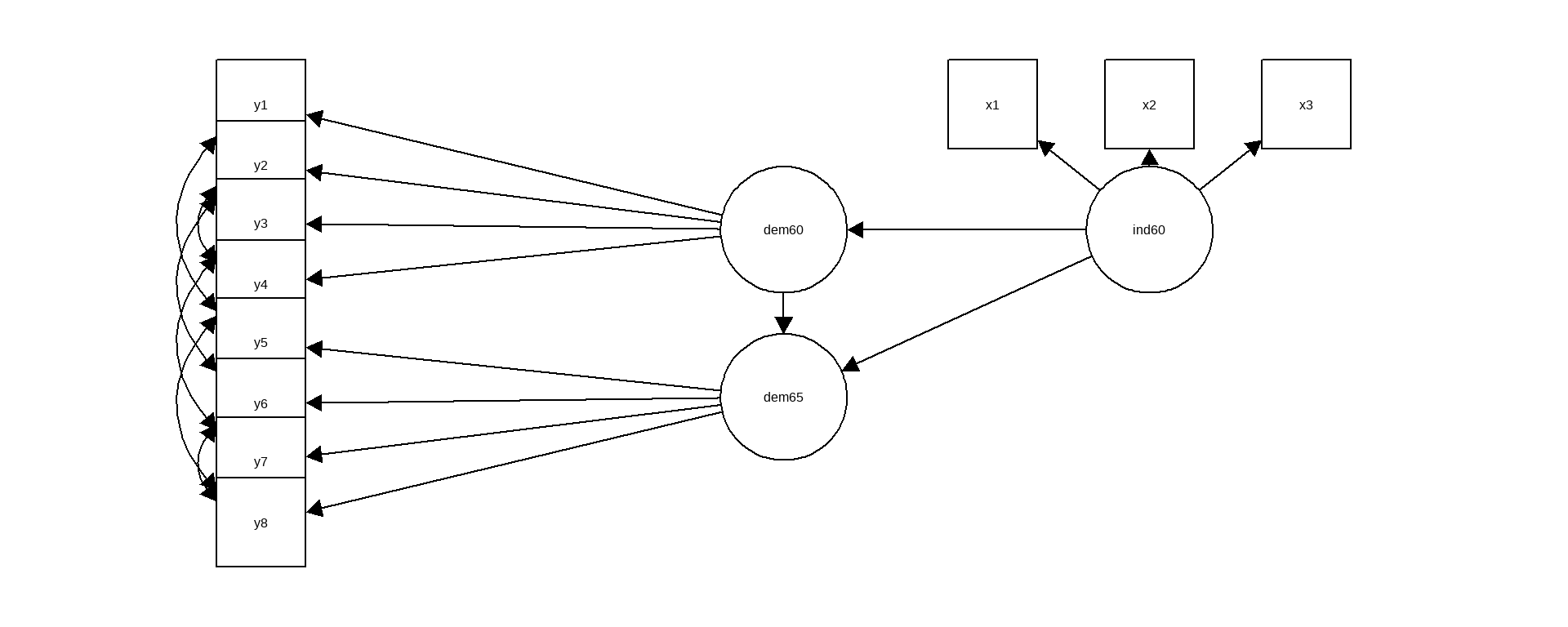
3.14 🌰 Bollen 1989

政治民主（1960，1965）与工业化

3.15 结果与诊断

lavaan 0.6-19 ended normally after 68 iterations

  Estimator                                         ML
  Optimization method                           NLMINB
  Number of model parameters                        31

  Number of observations                            75

Model Test User Model:
                                                      
  Test statistic                                38.125
  Degrees of freedom                                35
  P-value (Chi-square)                           0.329

Model Test Baseline Model:

  Test statistic                               730.654
  Degrees of freedom                                55
  P-value                                        0.000

User Model versus Baseline Model:

  Comparative Fit Index (CFI)                    0.995
  Tucker-Lewis Index (TLI)                       0.993

Loglikelihood and Information Criteria:

  Loglikelihood user model (H0)              -1547.791
  Loglikelihood unrestricted model (H1)      -1528.728
                                                      
  Akaike (AIC)                                3157.582
  Bayesian (BIC)                              3229.424
  Sample-size adjusted Bayesian (SABIC)       3131.720

Root Mean Square Error of Approximation:

  RMSEA                                          0.035
  90 Percent confidence interval - lower         0.000
  90 Percent confidence interval - upper         0.092
  P-value H_0: RMSEA <= 0.050                    0.611
  P-value H_0: RMSEA >= 0.080                    0.114

Standardized Root Mean Square Residual:

  SRMR                                           0.044

Parameter Estimates:

  Standard errors                             Standard
  Information                                 Expected
  Information saturated (h1) model          Structured

Latent Variables:
                   Estimate  Std.Err  z-value  P(>|z|)
  ind60 =~                                            
    x1                1.000                           
    x2                2.180    0.139   15.742    0.000
    x3                1.819    0.152   11.967    0.000
  dem60 =~                                            
    y1                1.000                           
    y2                1.257    0.182    6.889    0.000
    y3                1.058    0.151    6.987    0.000
    y4                1.265    0.145    8.722    0.000
  dem65 =~                                            
    y5                1.000                           
    y6                1.186    0.169    7.024    0.000
    y7                1.280    0.160    8.002    0.000
    y8                1.266    0.158    8.007    0.000

Regressions:
                   Estimate  Std.Err  z-value  P(>|z|)
  dem60 ~                                             
    ind60             1.483    0.399    3.715    0.000
  dem65 ~                                             
    ind60             0.572    0.221    2.586    0.010
    dem60             0.837    0.098    8.514    0.000

Covariances:
                   Estimate  Std.Err  z-value  P(>|z|)
 .y1 ~~                                               
   .y5                0.624    0.358    1.741    0.082
 .y2 ~~                                               
   .y4                1.313    0.702    1.871    0.061
   .y6                2.153    0.734    2.934    0.003
 .y3 ~~                                               
   .y7                0.795    0.608    1.308    0.191
 .y4 ~~                                               
   .y8                0.348    0.442    0.787    0.431
 .y6 ~~                                               
   .y8                1.356    0.568    2.386    0.017

Variances:
                   Estimate  Std.Err  z-value  P(>|z|)
   .x1                0.082    0.019    4.184    0.000
   .x2                0.120    0.070    1.718    0.086
   .x3                0.467    0.090    5.177    0.000
   .y1                1.891    0.444    4.256    0.000
   .y2                7.373    1.374    5.366    0.000
   .y3                5.067    0.952    5.324    0.000
   .y4                3.148    0.739    4.261    0.000
   .y5                2.351    0.480    4.895    0.000
   .y6                4.954    0.914    5.419    0.000
   .y7                3.431    0.713    4.814    0.000
   .y8                3.254    0.695    4.685    0.000
    ind60             0.448    0.087    5.173    0.000
   .dem60             3.956    0.921    4.295    0.000
   .dem65             0.172    0.215    0.803    0.422

3.16 小结

• CFA
  • 验证性因子分析：检验潜在变量对于观察指标是否有影响
  • CFA诊断：χ², TLI/CFI，RMSEA/SRMR

• SEM
  • Latent + measurement models
  • 不能证明因果关系！