


数据可视化理论与工具
政务大数据应用与分析 (80700673)
1.2 A Picture is Worth a Thousand Words
Even before he became president, Mr Trump had a history of controversial comments about women. His comments in a 2005 Access Hollywood tape about grabbing women “by the pussy” are perhaps the most notorious, and made headlines in 2016…..”The kind of things that he said about Hillary Clinton, Carly Fiorina, Elizabeth Warren, Heidi Cruz—the list goes on—he talks about women, any prominent, powerful woman, in the most DEMEANING of ways, trivializing them.”(Rogers 2016)

1.3 可视化与人类技术发展

1.4 可视化与政治学研究
Kastellec and Leoni (2007): APSR,AJPS和PA 2006年五刊

1.5 表转图

下面的可视化做得如何


1.6 “毒图”(Viral Charts)


1.7 图的问题也是人的问题


1.8 如何识别“毒图” (Smith 2023, 2024)
- 🚩 Startling trend
- 🚩 Unlabeled/Dual axis
- 🚩 No source
- 👁️ Learn about old tricks
- 👁️ Check comments
- 👁️ Check where axis starts
- 👁️ Check the unit of axes
1.9 做幅合格的图
如何可视化以下数据?
| 政党 | 得票率 |
|---|---|
| A | 38 |
| B | 34 |
| C | 24 |
| D | 4 |
1.10 什么是不合格的图
- 使用多种图形组成要素重复呈现同一种信息
- 虽未歪曲数据,但可能误导读者


1.11 Quiz 1


1.12 Call back

1.14 下列数据如何可视化?
| Party | PRI | PAN | PRD | Others |
|---|---|---|---|---|
| 1991 | 64 | 17.8 | 8.2 | 10 |
| 1994 | 60 | 23.8 | 14.2 | 2 |
| 1997 | 47.8 | 24.2 | 25 | 3 |
| 2000 | 42.2 | 41.2 | 10 | 6.6 |
| 2003 | 44.8 | 30.2 | 19.4 | 5.6 |
和之前的数据有什么不同?
堆积图

1.15 其他选择


1.16 不是越简单越好


Pro
- 散点图变异
- 通过气泡大小呈现第三维度数据
Con
- 气泡大小当接近时可能造成辨识困难,信息无法完全精确地传达
2.1 可视化编码
- 数值(numeric)
- 10厘米,17厘米,23厘米
- 定序(ordinal)
- 小,中,大
- 周日,周一,周二……
- 定类(nominal)
- 苹果,桔子,香蕉……
标记:点、线、面
![]()
通道:位置、大小、形状、方向、色调、饱和度、亮度……
![]()


2.2 通道


2.4 什么叫有效性


2.5 准确性(Accuracy)
\[\displaystyle S (I)=kI^{n},\]
k: proportionality constant that depends on the units used

2.6 可辨性(Discriminability)


2.7 可分离性(Separability)

2.8 视觉突出(Pop-out)


2.9 视觉突出基础:分主次


2.10 通过分组分主次
- 分组会对大部分任务有效
- 如果不能进行分组,则需要转换任务目标
- 避免过多类别
- 对数据的每个维度指定一种或一个阶层的颜色

2.11 色彩
- 灰度有序 → 数值型
- 色调无序 → 类别型


色彩设计基本原则
- 避免过多颜色交错导致的杂乱无章
- 注意控制同时对比(Simultaneous contrast)
- 注意饱和度


Warning
入门容易,坑较深(没大必要入)
2.13 调色板


2.14 向大厂学习


2.17 Take-Home Points
可视化理论
- 抉择:精确 vs. 眼球
- 可视化基本原则
- 准确
- 明确
- 详确
可视化工具
- 编码和通道
- 通道选择原则
- 有效性
- 准确性
- 表现力
- 可辨性
- 可分离性
- 视觉突出
- 有效性
- 色彩
- 相信专家
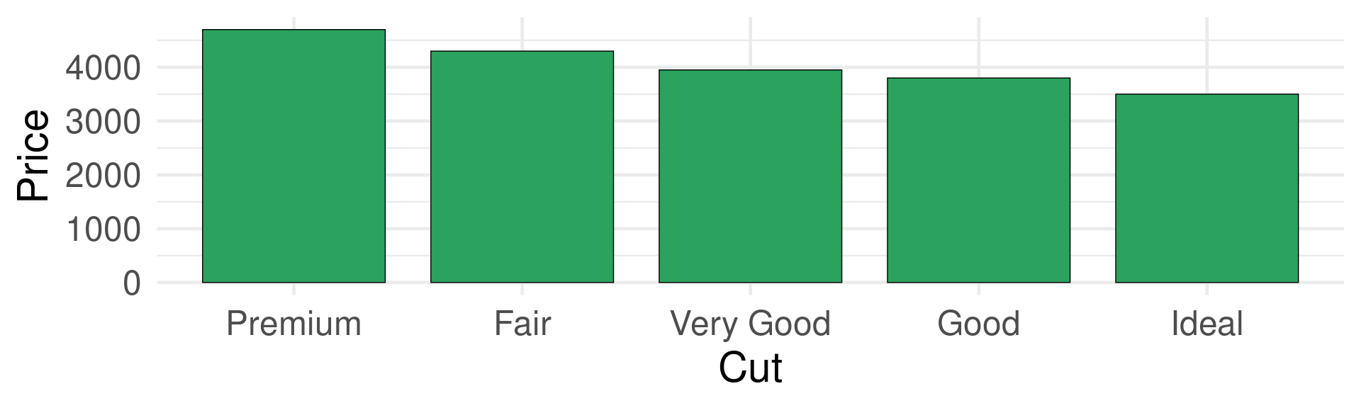
3.2 描述图:柱状图
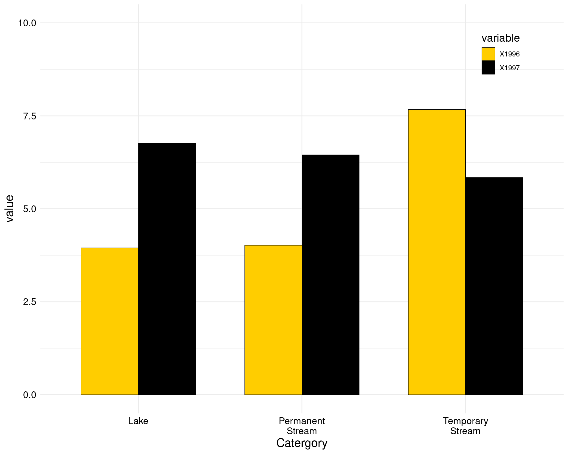
3.3 分组柱状图
ggplot(data = mydata2,
       aes(Catergory, value,
           fill = variable)) +
  geom_bar(
    stat = "identity",
    color = "black",
    position = position_dodge(),
    width = 0.7,
    size = 0.25
  ) +
  drhutools::scale_fill_gb() +
  theme_minimal() +
  ylim(0, 10) +
  theme(
    axis.title = element_text(size = 15, face = "plain", color = "black"),
    axis.text = element_text(size = 12, face = "plain", color = "black"),
    legend.title = element_text(size = 14, face = "plain", color = "black"),
    legend.background  = element_blank(),
    legend.position = c(0.88, 0.88)
  )
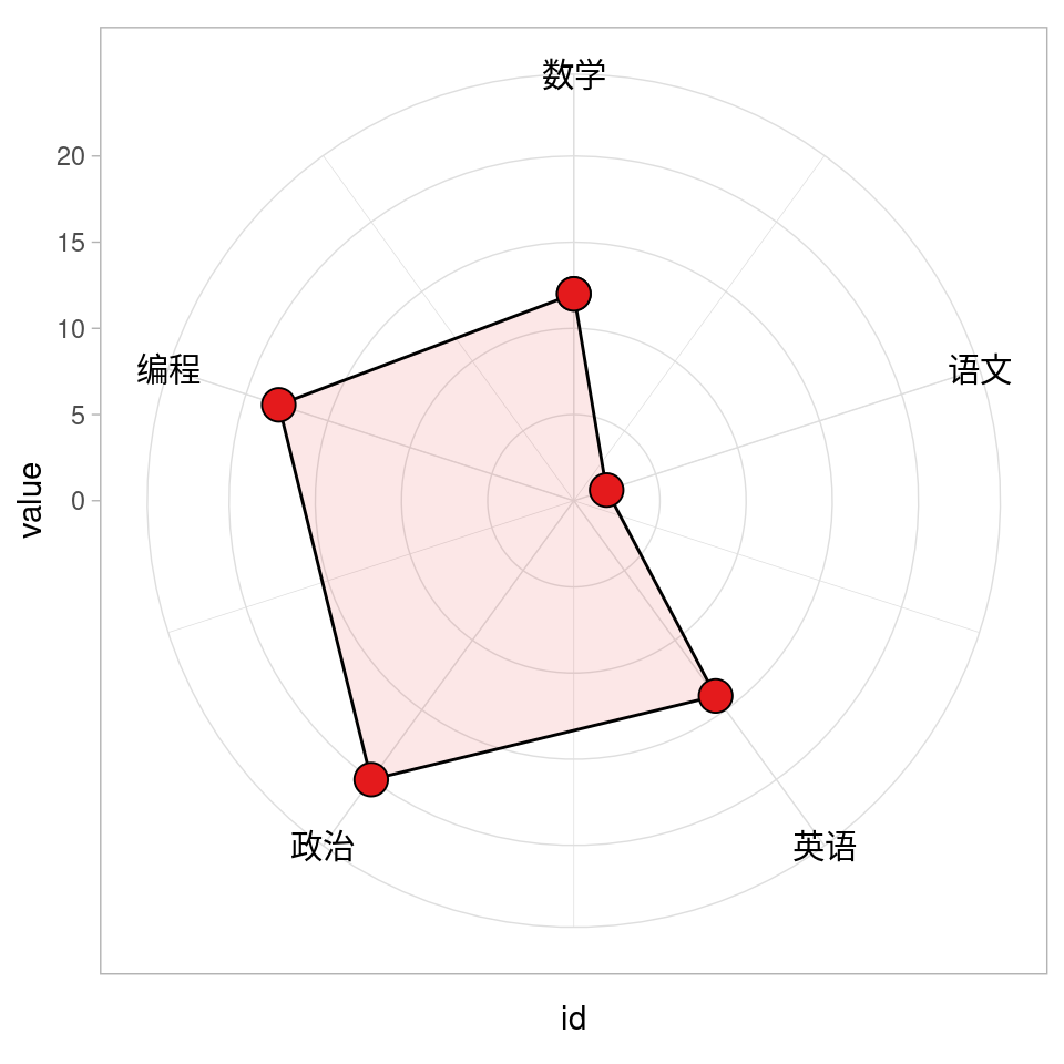
ggplot() +
  geom_polygon(
    data = mydata,
    aes(x = id, y = value),
    color = "black",
    fill = brewer.pal(7, "Set1")[1],
    alpha = 0.1
  ) +
  geom_point(
    data = mydata,
    aes(x = id, y = value),
    size = 5,
    shape = 21,
    color = 'black',
    fill = brewer.pal(7, "Set1")[1]
  ) +
  coord_radar() +
  scale_x_continuous(breaks = label_data$id, labels = label_data$car) +
  ylim(0, 22) +
  theme_light() +
  theme(axis.text.x = element_text(
    size = 11,
    colour = "black"
  ))
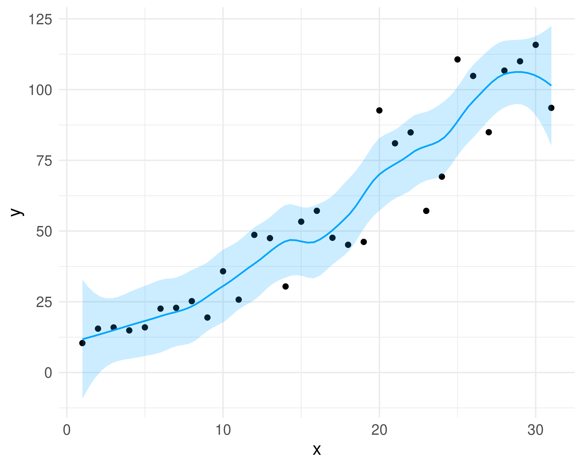
3.5 描述图:趋势图(点-线)
ggplot(data = mydata, aes(x, y)) +
  geom_point(
    fill = "black",
    colour = "black",
    size = 3,
    shape = 21
  ) +
  geom_smooth(
    method = 'loess',
    span = 0.4,
    se = TRUE,
    colour = "#00A5FF",
    fill = "#00A5FF",
    alpha = 0.2
  ) +
  scale_y_continuous(breaks = seq(0, 125, 25)) +
  theme(
    text = element_text(size = 15, color = "black"),
    plot.title = element_text(
      size = 15,
      family = "myfont",
      hjust = .5,
      color = "black"
    ),
    legend.position = "none"
  )
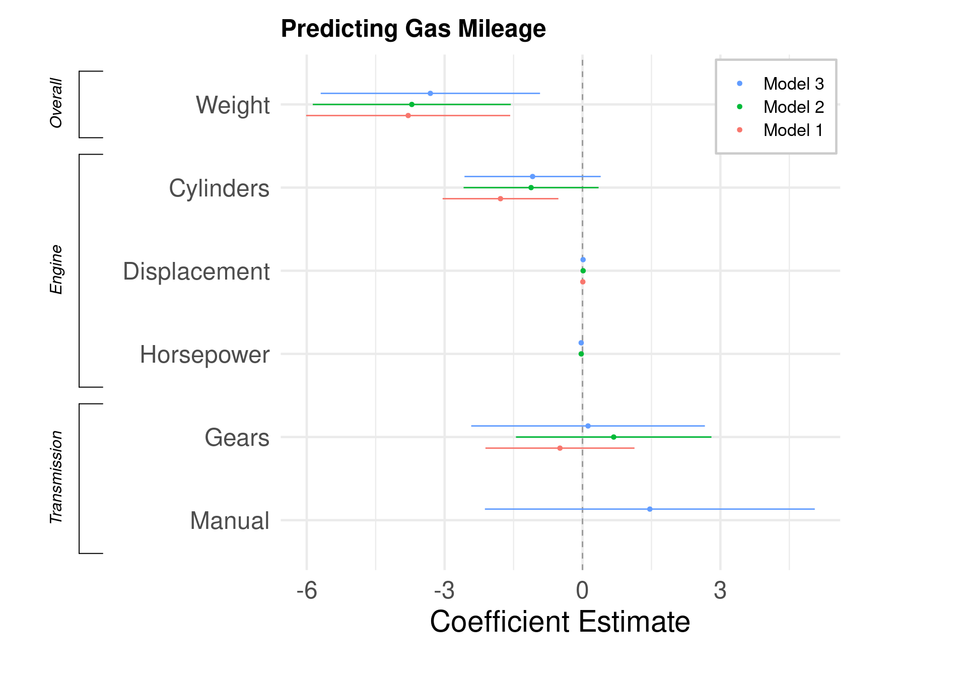
3.7 Dot-whisker

3.8 More delicate version
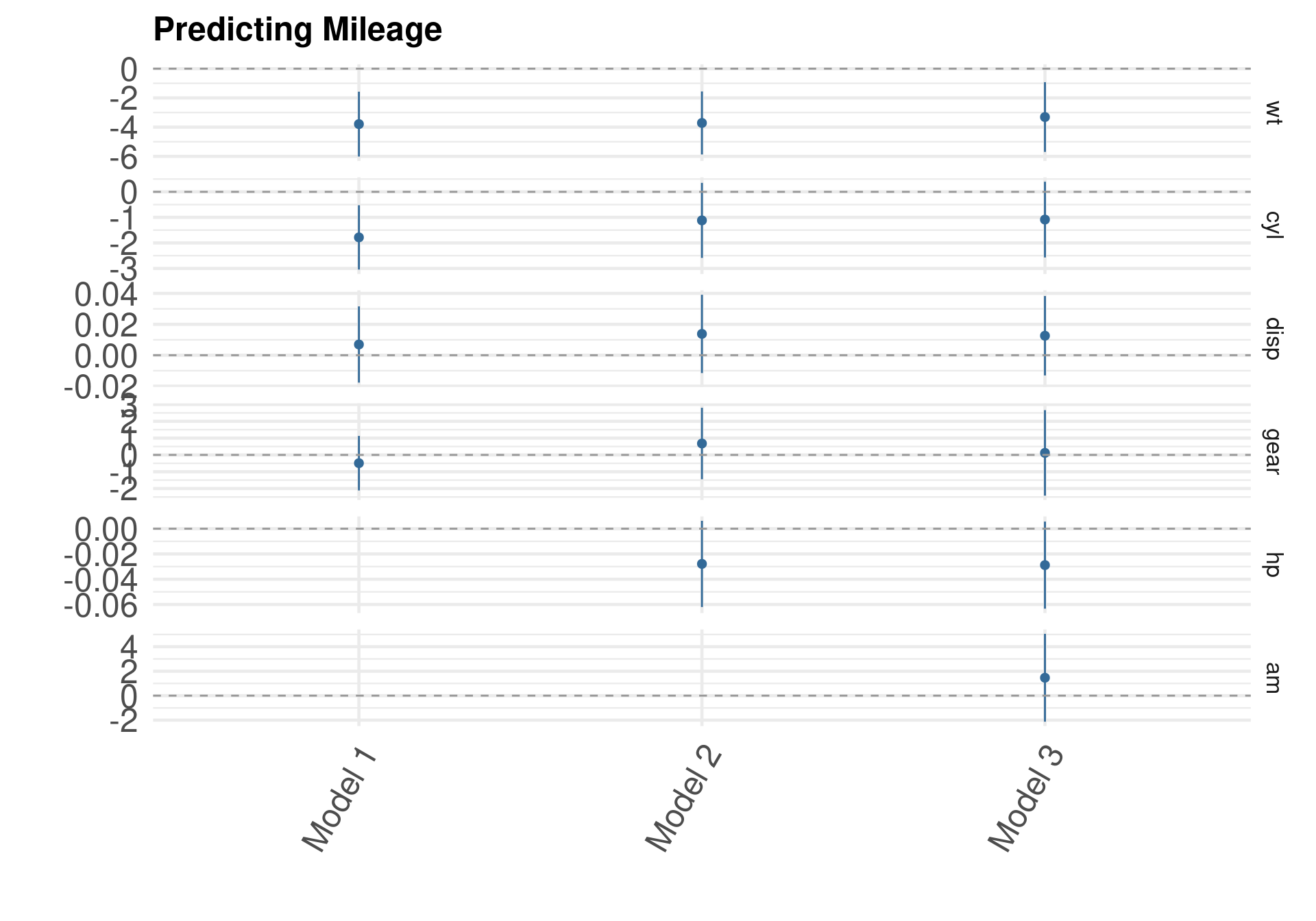
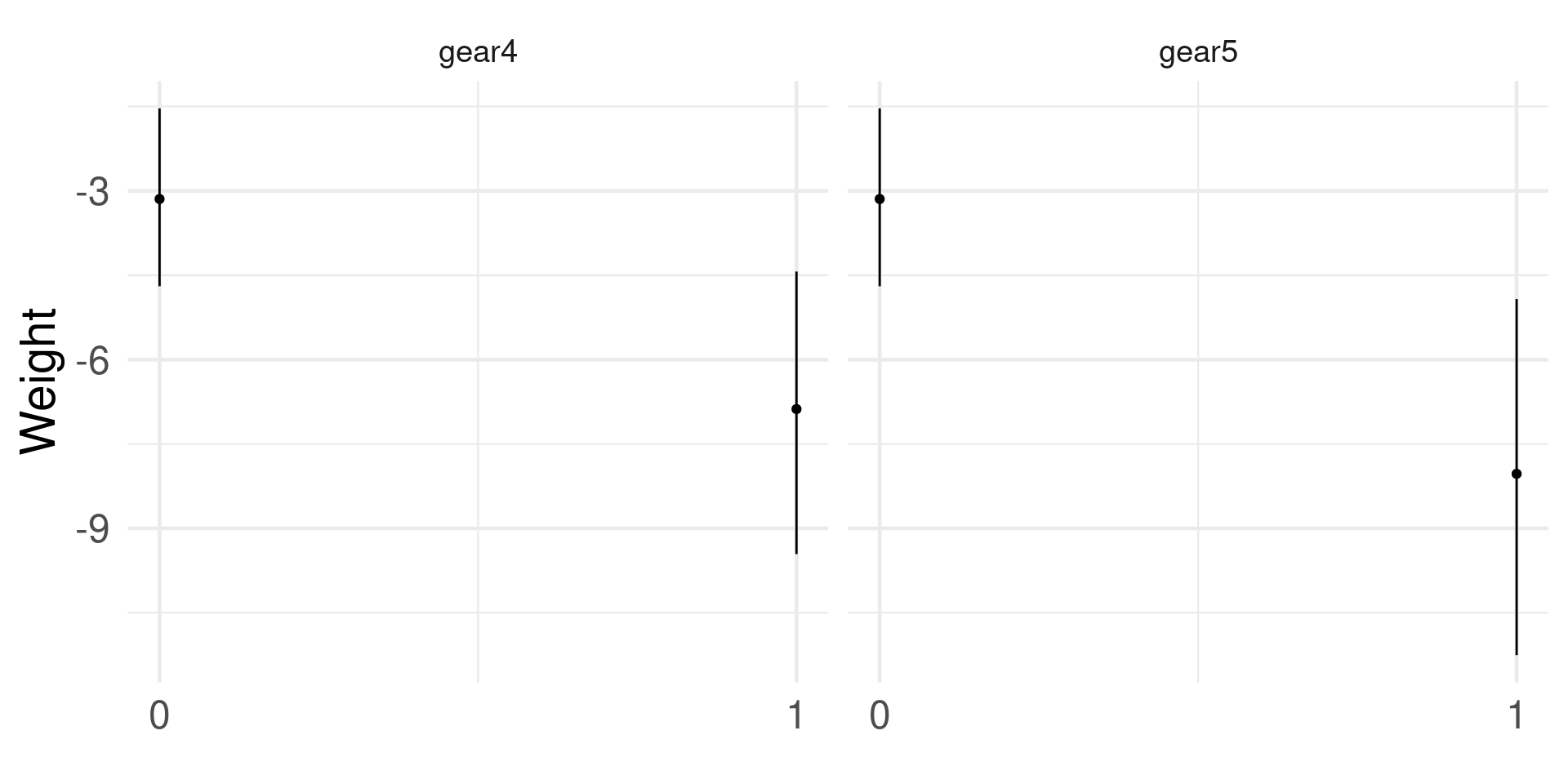
3.9 Small-multiple
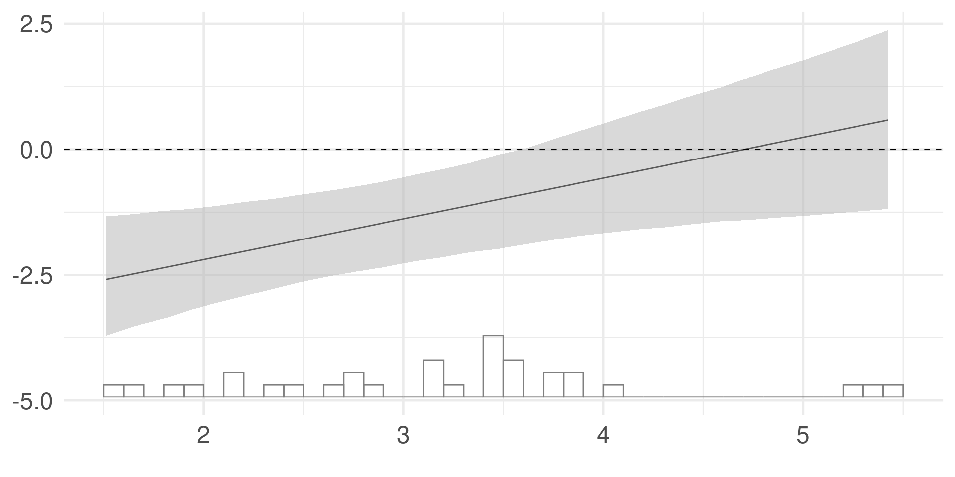
3.10 结果图:交互效应(interplot)
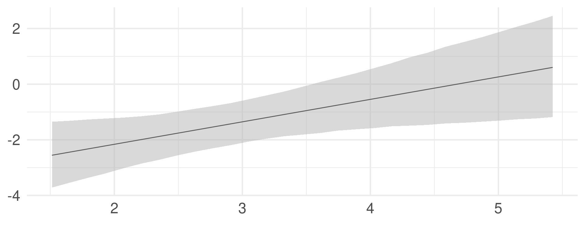
3.11 More delicate
3.12 描述性统计
| Unique | Missing Pct. | Mean | SD | Min | Median | Max | Histogram | |
|---|---|---|---|---|---|---|---|---|
| mpg | 25 | 0 | 20.1 | 6.0 | 10.4 | 19.2 | 33.9 |  |
| cyl | 3 | 0 | 6.2 | 1.8 | 4.0 | 6.0 | 8.0 |  |
| disp | 27 | 0 | 230.7 | 123.9 | 71.1 | 196.3 | 472.0 |  |
| hp | 22 | 0 | 146.7 | 68.6 | 52.0 | 123.0 | 335.0 |  |
| drat | 22 | 0 | 3.6 | 0.5 | 2.8 | 3.7 | 4.9 |  |
| wt | 29 | 0 | 3.2 | 1.0 | 1.5 | 3.3 | 5.4 |  |
| qsec | 30 | 0 | 17.8 | 1.8 | 14.5 | 17.7 | 22.9 |  |
| carb | 6 | 0 | 2.8 | 1.6 | 1.0 | 2.0 | 8.0 |  |
| N | % | |||||||
| vs | FALSE | 18 | 56.2 | |||||
| TRUE | 14 | 43.8 | ||||||
| am | FALSE | 19 | 59.4 | |||||
| TRUE | 13 | 40.6 | ||||||
| gear | 3 | 15 | 46.9 | |||||
| 4 | 12 | 37.5 | ||||||
| 5 | 5 | 15.6 |