Principles of
Text Analysis

Data Science and Text Analysis, CAMS, CityU

Yue Hu

Department of Political Science

Tsinghua University

Outline

• Text-As-Data Approach
• DGP for Text-As-Data
• Analyzing text data

Text-As-Data Approach

Text: the oldest data

Long before spreadsheets, humanity stored its records in words.

• Cuneiform in Mesopotamia (~3200 BCE)
• Egyptian hieroglyphs
• Oracle-bone script of Shang-dynasty China

Text is the oldest form of “data storage”

—and still the richest record of human life.

Every language is an application programming interface (API).

When text becomes (big) data

More text is produced each day than any of us could read in a lifetime:

• Email: 36+ billion messages sent and received every day worldwide.
• WeChat: 45+ billion messages a day—1.5+ TB of new data daily.
• Social media: tens of thousands of new posts every second.

These oceans of text carry attitudes, emotions, values, political stances—even consumer preferences.

By 2020, the size of global data has reached 40ZB (5.2TB/person).¹

http://pdf.dfcfw.com/pdf/H3_AP201903111304577789_1.pdf

Giga Byte < Tera Byte < Peta Byte < Exa Byte < Zetta Byte < Yotta Byte

1. ¹ 1ZB = 1,024EB = 1,024²PB = 1,024³TB = 1024⁴GB—reference: 1080p HD 2hrs：6GB

A long tradition of reading text

East

• Exegesis (訓詁學): Erya, Shuowen Jiezi
• Evidential scholarship (考據學) of the Qing

West

• Greek rhetoric
• Biblical hermeneutics
• 19th-century philology

Toward science: Lasswell’s content analysis of wartime propaganda (1927); Stone’s General Inquirer, the first computer text analysis (1962).

Before computers: four hard limits

• Early empirical uses of text
  • Law and the externality problem (Coase 1960)
  • Policy surprises from historical documents (Friedman and Schwartz 2008)

• Why systematic analysis stayed out of reach:
  1. Preservation & updating — documents decay; ephemera are lost
  2. Subjectivity — no shared, replicable coding standard
  3. Time cost — even a handful of texts takes enormous effort
  4. Limited inference — case studies rarely generalize

→ Early work was confined to close reading of a few classics.

The two examples both treat text as evidence, long before “text as data” was a method.

• Coase (1960), “The Problem of Social Cost”: Coase builds his argument by reading actual court cases—rulings on straying cattle, a factory’s smoke, a confectioner’s noise disturbing a doctor. The legal records are his data. From these documents he derives what became the Coase theorem: when transaction costs are low, parties bargain to an efficient allocation of rights regardless of who is initially liable. Externalities are read out of legal text, not modeled from assumptions.

• Friedman & Schwartz (2008 [1963]), A Monetary History of the United States, 1867–1960: They assemble nearly a century of historical records—Federal Reserve minutes, bank reports, policy documents—to reconstruct the money supply. Reading these documents overturned the received story of the Great Depression: the collapse was deepened by the Fed’s contraction of the money supply, a policy “surprise” that only surfaces once you work through the archival paper trail.

The computational turn

Three shifts opened the floodgates from the 1990s on:

1. Democratized data — blogs, forums, social media: ordinary voices, not just elite texts.
2. Computational methods — NLP and machine learning automate topic, sentiment, and extraction.
3. Mature theory — Grimmer & Stewart (2013), and later Grimmer et al. (2022), laid the “text as data” foundation.

Why compute? (Not just “big data”)

Not only because we can handle more data

Three reasons size alone is not the justification:

1. Bigger ≠ better
2. Language breaks the independence assumption
3. Machines read backwards from humans

Three uncomfortable truths

• Bigger ≠ better
• Independence
• Backwards

Large samples indeed help in classical statistics via the law of large numbers, but

• What is the population of a language?
  • One person’s words? A nation’s? All of humanity’s?
• Language is open and ever-generating with no clear boundary (Biber 1993).
  • Size alone guarantees no representativeness.

Most statistics assume independent units, but

• Language is the opposite
  • “he” needs an antecedent;
  • “however” presupposes a claim to overturn
• Meaning is nested from character to word to sentence to document.
  • Counting words as if they were independent throws away the essence.

• No one writes by sampling words from a corpus by probability;
• No one reads by tallying every word before forming a view
• Human language is real-time, situated, goal-directed.

The computer must do the reverse: gather everything first, then hunt for patterns.

Then what are we hunting?

Statistical regularities the naked eye cannot see.

Zipf’s law: in any large text, frequency is inversely proportional to rank: the 2nd word appears about half as often as the 1st, the 3rd about a third as often… strikingly stable across languages (Zipf [1949] 2016).

• Function words — pronouns, prepositions, conjunctions:
  • Used almost unconsciously, yet betray attention, emotion, and social relations (Pennebaker 2017).

Example: Heavy use of “I” tracks depression; the emotional tone of Justices’ words in oral argument even predicts their votes (Black et al. 2011; Liu 2022).

Text-as-data perspective

Objective

Text Language

Terminology

• Text analysis vs. content analysis
• Representational vs. Instrumental
• Thematic vs. semantic

Representational 精确解码，关注外显（manifest）； Instrumental 探索意图，关注隐含（latent） Thematic 概念是否出现及何种关系，基于词频和向量； Semantic 识别主题间的具体关系；考虑语法、逻辑等

语法学(syntax, how to say it) 语义学(semantic, what is said) 语用学(pragmatic, what is implicated)

Approach

	Content analysis	Discourse analysis	Computational
Core question	What is said?	How & why said?	What statistical regularities?
Scale	Small–mid	Small	Large
Main tool	Human coding	Qualitative reading	Algorithms
Strength	Replicable, objective	Deep, context-sensitive	Efficient; finds hidden patterns
Limit	Codebook-bound, hard to scale	Subjective, hard to generalize	May lose context

Illustration I

Grimmer (2010)

• Objective
  • The priorities political actors emphasize in statements
• Data
  • An original collection of over 24,000 Senate press releases in 2007
• Method
  • Bayesian Hierarchical Topic Model

Findings

• Focus
• Cluster
• Predict

Committee leaders focus on their committee’s issues

Fig. 4 Chairman and ranking members of committees allocate more attention to issues under their committees’ jurisdiction than other senators. This figure compares the attention that Senate committee leaders—chairs or ranking members—dedicate to topics under their committee jurisdictions to the attention allocated by the rest of the Senate. The solid dots represent the expected difference, the thick lines are 80% credible intervals, and the thin lines are 95% intervals. Along the left-hand vertical axis, the topics are listed, and on the right-hand side, the corresponding committee names are listed. In all but seven cases, the dot is to the right of the zero line, indicating that leaders of committees discuss issues that highlight their power in the institution more often than other senators.

Expressed agendas cluster geographically

Fig. 5 Attention to issues follows expected geographic patterns. This figure demonstrates that senators’ expressed agendas are grouped geographically. The left-hand plot shows that senators from western states allocate substantial attention to public-land issues. Darker shades indicate that the average expected attention from the state’s delegation to public-land issues is larger. The center plot carries out a comparison of three different regional issues: public-land and western states (top estimate), hurricanes and gulf coast states (middle estimate), and border-security and states that share an international border (bottom estimate). The point in each plot represents the expected difference between the attention senators in a geographic area allocate to an issue and the attention senators from other areas of the country dedicate to the same issue. The thick and thin lines are 80% and 95% HPD intervals for this difference. Each point is to the right of the zero, indicating that the issues receive more attention in the geographic areas we would expect. The right-hand plot shows that senators from states with a large number of farms per person also tend to allocate more attention to agriculture issues. The horizontal axis represents the number of farms per resident of the state (one measure of agriculture’s importance to a state), and the vertical axis indicates the proportion of press releases allocated to agricultural issues. The gray lines are lowess curves indicating the relationship between the number of farms per capita and the attention to agriculture, whereas the black line is the average relationship.

Attention to appropriations predicts opposition to earmark reform

An earmark is a provision inserted into a discretionary spending appropriations bill that directs funds to a specific recipient while bypassing the merit-based or competitive funds allocation process. These provisions are often associated with legislation specifying certain congressional spending priorities or in revenue bills that apply to a limited number of individuals or entities.

The DeMint-McCain amendment was a significant proposal related to earmark reform. Senator Jim DeMint introduced a one-year earmark moratorium amendment, which was co-sponsored by both Republicans and Democrats. The amendment aimed to end the era of earmarks and was seen as a step towards increased transparency, accountability, and fiscal responsibility in Congress. Despite its support from some senators and advocacy groups, the amendment was defeated in a late-night Senate vote, with a result of 29-71.

Fig. 6 Senators who dedicate more attention to appropriations were more likely to oppose DeMint-McCain. This figure shows that senators who dedicate more attention to appropriations in their press releases are more likely to oppose the DeMint-McCain amendment. The vertical axis plots the vote on the amendment, and along the horizontal axis is the average proportion of press releases dedicated to discussing appropriations secured for fire departments. To generate the light gray lines, I took 100 draws from each senator’s posterior expressed agenda and then regressed the earmark vote on the draw from the posterior. The gray lines represent the expected probability of supporting the DeMint-McCain amendment, and the solid black line is the expected value of the relationship, averaged over the draws from the posterior distribution on the expressed agenda.

The left-hand figure shows that senators who discuss fire department grants more often were more likely to oppose the DeMint-McCain amendment, and the center plot shows that this relationship was even stronger for an aggregate appropriations category. The right-hand plot shows that the relationship remains even after conditioning upon estimated ideal points of senators, suggesting that consistency explains components of voting behavior beyond ideal point estimates.

Illustration II

Benoit et al. (2016)

• Objective
  • Professionals vs. Masses
• Method
  • Crowd-sourced identification
• Data
  • 18,263 natural sentences from British Conservative, Labour and Liberal Democrat manifestos

Operation

• Coding
• Results

Figure 1: Hierarchical coding scheme for two policy domains with ordinal positioning.

Figure 2. British party positions on economic and social policy 1987 – 2010; sequential expert text processing (vertical axis) and independent expert surveys (horizontal).

Illustration III

Dietrich et al. (2019)

• Objective
  • Speakers’ emotional state
• Method
  • Analyses of vocal pitch
• Data
  • 74,158 Congressional floor speeches

Operation

Illustration IV

Zhang and Pan (2019)

• Objective
  • Group activities from social media
• Method
  • CNN for images; CNN-RNN for texts
• Data
  • A random sample of 20,000 geocoded posts from Weibo, 2010–2017

CNN: Convolutional Neural Network

RNN: Recurrent Neural Network

Operation

Challenges

Theory

• Single causal mechanism?
  • Intentional writing vs. measurement errors

Assumption

• A bag of words (elaborated later)

Data

• Unstructured data
• Manifest and latent dimension reduction
• Concept relations and context ignorance
• DGP
  • Only posted
  • One-time censor?
  • Random sampling?

审查已经使用 machine learning Su et al. (2020)

Wrap it up

• History of text-as-data
  • Long and short
• Text-as-data perspectives
  • Objective: language
  • Types
• Application
  • Text → audio, video

DGP for Text-As-Data

Points to cover

1. Where to find text resources?
   1. First-hand sources
   2. Second-hand sources
2. How to get text resources?
3. How to deal with text information?
4. What can text data do?

First-hand sources

Text from authors

• Email/SMS
• Website HTML
• RSS feeds
• Internet social media
• Internet Forum
• Network question and answer platform
• Media database
• Internet transaction behavior
  ……

Open Platforms

Media database

E-Government

Social Media

新浪微博1.4亿，微信用户5.5亿; 微信日增数据500TB，QQ日增数据200TB。

Reddit

Quora, Stack Overflow

Open question

Second-hand sources

Text from archives

• CNKI and other databases (journals, newspapers, yearbooks, etc.)
• Google Books, Baidu Scholar
• Google Trend, Baidu Index
• JSTOR Data for Research
  ……

Indicators

Digitalized documents

Text data collection

• First-hand: Spider/crawler/scraper
• Second-hand: archive and digital database

Scraper operation

Customized Scraping

SelectorGadget (Chrome extension)

Scraping with rvest

ls_zhongsheng <-
  read_html("http://politics.people.com.cn/GB/8198/426918/index.html") |> # index page
  html_nodes("h5 a") |> # the nodes of the links
  html_attr("href") |> # just the links
  str_replace("^/n1", "http://politics.people.com.cn/n1")

df_zhongsheng <- map_df(ls_zhongsheng, function(link) {
  zs_article <- read_html(link, encoding = "GB18030") # read the html

  zs_title <- html_nodes(zs_article, "h1") |>
    html_text

  zs_time <- html_nodes(zs_article, ".box01 .fl") |>
    html_text |>
    str_extract("\\d{4}年\\d{2}月\\d{2}日")

  zs_content <- html_nodes(zs_article, "#rwb_zw p") |>
    html_text |>
    str_c(collapse = "") |> # combined the paragraphs
    str_remove_all("\\s|\\n|\\t") # remove the horizontal spaces

  zs_data <- data.frame(title = zs_title, time = zs_time, content = zs_content)
})

Regular Expression

Structuralization

Wrap it up

• Source of text data
  • First-hand
  • Second-hand
• Data collection
  • First-hand: Scraping
    • Foolproof software
    • Programming
      • Regular expression
  • Second-hand: Archives
• Structuralization

Analyzing text data

An (Classic) Overview (Grimmer and Stewart 2013)

Level of Analysis

Description

Frequency, word cloud (👎), network

Classification

Supervised, unsupervised, self-supervised

Semantics

Sentiment analysis, word embedding, word sequence, relationship

Tenet of Text-as-data analysis (Grimmer and Stewart 2013)

1. All quantitative models of language are wrong—but some are useful.
2. Quantitative methods for text amplify resources and augment humans.
3. There is no globally best method for automated text analysis.
4. Validate, Validate, Validate.

The human stays in the loop

The computer computes; the researcher reasons.

Only you can:

• Ask a question worth asking
• Choose fit-for-purpose data & methods
• Interpret what a pattern means
• Put findings in dialogue with theory
• Name the limits of the conclusion

Unit of Analysis

• Corpus
  • Document (volume, chapter, section)
    • Paragraph
      • Sentence ✓
        • Clause ✓
          • Word (Unigram) ✓
            • Token ✓

Token

Sequence of linguistic features

• Token in a document: term
• Token in a group: N-gram
  • A word = a Unigram

Unrealistic Assumption

Where the “all models are wrong” starts

Bag of words (BoW)

A text is represented as the bag (multiset) of its words.

From natural language to computational language

Document-Term Matrix (DTM)

In linguistics, the opposite of natural language is artificial/constructed language (conlangs), like Klingon in “Star Trek,” Dothraki in “Game of Thrones”

Preprocessing

• Segmentation
• Tokenization
• Stopwords/function words removal
• Other project-oriented wrangling

Segmentation

Scriptio discreta (e.g., English)

Document → paragraphs/sentences

discrete script

Scriptio continua (e.g., CJK)

library(jiebaR)

zhongsheng <- "近年来，美国一些政客被“美国优先”遮住了双眼，大搞贸易保护主义、单边主义，肆意挥舞关税大棒，全然不顾中美两国人民和全世界人民的强烈反对。"
cutter <- worker() # segment engine

segment(zhongsheng, cutter)

 [1] "近年来"   "美国"     "一些"     "政客"     "被"       "美国"    
 [7] "优先"     "遮住"     "了"       "双眼"     "大"       "搞"      
[13] "贸易"     "保护主义" "单边主义" "肆意"     "挥舞"     "关税"    
[19] "大棒"     "全然不顾" "中美"     "两国人民" "和"       "全世界"  
[25] "人民"     "的"       "强烈"     "反对"    

continuous script

《人民日报》（2019年05月30日02版）

Tokenization

• Goal: Removing syntax
• Removing: capitalization, punctuation, non-alphanumeric characters (@#$%……&*), stop words

Examples of Stopwords

 [1] "to"     "can"    "could"  "dare"   "do"     "did"    "does"   "may"   
 [9] "might"  "would"  "should" "must"   "will"   "ought"  "shall"  "need"  
[17] "is"     "a"      "am"     "are"    "about" 

 [1] "一些"   "一何"   "一切"   "一则"   "一方面" "一旦"   "一来"   "一样"  
 [9] "一般"   "一转眼" "万一"   "上"     "上下"   "下"     "不"     "不仅"  
[17] "不但"   "不光"   "不单"   "不只"   "不外乎"

Stopwords sources for Chinese

• 百度停词表
• 哈工大停词表
• 网络搜集停词表，如“最全中文停用词表整理（1893个）”

Dimension reduction

Issue: Sparse matrix

• Lemmatization: (happy, happier, happiness) → happy
• Stemming: (happy, happier, happiness) → happi

More Examples

• Lemmatization: (went, leaves, geese, unhappy) → (go, leaf, goose, unhappy)
• Stemming: (went, leaves, geese, unhappy) → (went, leav, geese, unhappi)

• Labeling
  • Content vs. function
  • Linguistic features: n., v., adj., adv., prep., conj…….

A comprehensive application

2019-05-14 ~ 05-22: China-US trade war

Data collection

Raw Data

df_zhongsheng <- readRDS(url(
  "https://drhuyue.site:10002/sammo3182/data/zhongsheng.RDS"
))

df_zhongsheng$segmented <- map_chr(df_zhongsheng$content, function(content) {
  segment(content, cutter) |> paste(collapse = " ")
})

df_zhongsheng$phase <- "US_fail"
df_zhongsheng$phase[df_zhongsheng$time <= "2019-05-22"] <- "theory_test"
df_zhongsheng$phase[df_zhongsheng$time <= "2019-05-11"] <- "reassessment"
df_zhongsheng$phase[df_zhongsheng$time <= "2019-05-08"] <- "optimism"


df_token <- df_zhongsheng |>
  select(-content) |>
  unnest_tokens(word, segmented) # tokenization

# Show the word counts
select(df_token, -phase) |> head()

                                           title       time word
1 难道非要撞了南墙才回头——意孤行必将失败（钟声） 2019-05-30   一
2 难道非要撞了南墙才回头——意孤行必将失败（钟声） 2019-05-30   场
3 难道非要撞了南墙才回头——意孤行必将失败（钟声） 2019-05-30 经贸
4 难道非要撞了南墙才回头——意孤行必将失败（钟声） 2019-05-30 摩擦
5 难道非要撞了南墙才回头——意孤行必将失败（钟声） 2019-05-30   让
6 难道非要撞了南墙才回头——意孤行必将失败（钟声） 2019-05-30 世界

Removing the stopwords

# removing the stop words
df_stopWords <- tibble(word = read_lines(STOPPATH))

df_token <- df_token |>
  anti_join(df_stopWords)

select(df_token, -phase) |> head()

                                           title       time word
1 难道非要撞了南墙才回头——意孤行必将失败（钟声） 2019-05-30   场
2 难道非要撞了南墙才回头——意孤行必将失败（钟声） 2019-05-30 经贸
3 难道非要撞了南墙才回头——意孤行必将失败（钟声） 2019-05-30 摩擦
4 难道非要撞了南墙才回头——意孤行必将失败（钟声） 2019-05-30 世界
5 难道非要撞了南墙才回头——意孤行必将失败（钟声） 2019-05-30 看到
6 难道非要撞了南墙才回头——意孤行必将失败（钟声） 2019-05-30 一个

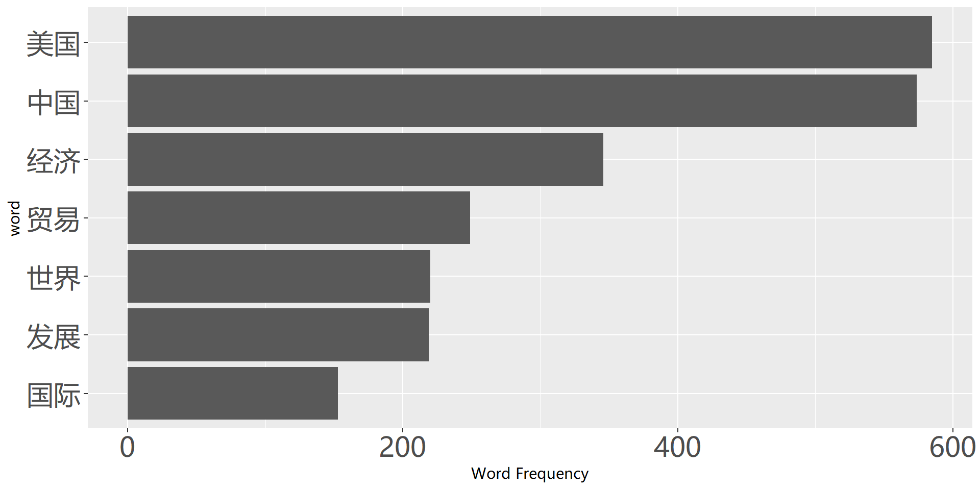
Frequency Analysis

df_plot <- df_token |>
  count(word, sort = TRUE) |>
  filter(n > 151) |>
  mutate(word = reorder(word, n))

ggplot(df_plot) +
  geom_col(aes(word, n)) +
  ylab("Word Frequency") +
  theme(axis.text = element_text(size = 20)) +
  coord_flip()

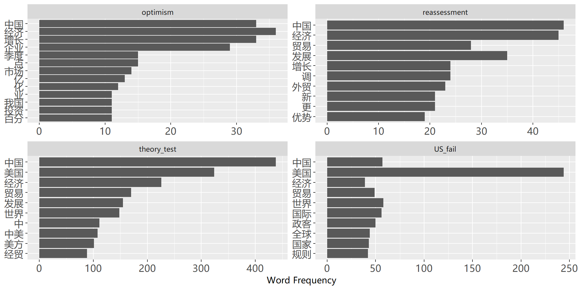
Frequency Dynamics

df_plot <- df_token |>
  group_by(phase) |>
  count(word, sort = TRUE) |>
  top_n(10) |>
  ungroup() |>
  mutate(
    word = reorder(word, n),
    word = factor(word, levels = rev(unique(word)))
  )

ggplot(df_plot, aes(word, n)) +
  geom_col() +
  xlab(NULL) +
  coord_flip() +
  ylab("Word Frequency") +
  theme(axis.text = element_text(size = 12)) +
  facet_wrap(~phase, scales = "free")

The Economist journalist Simon Rabinovitch

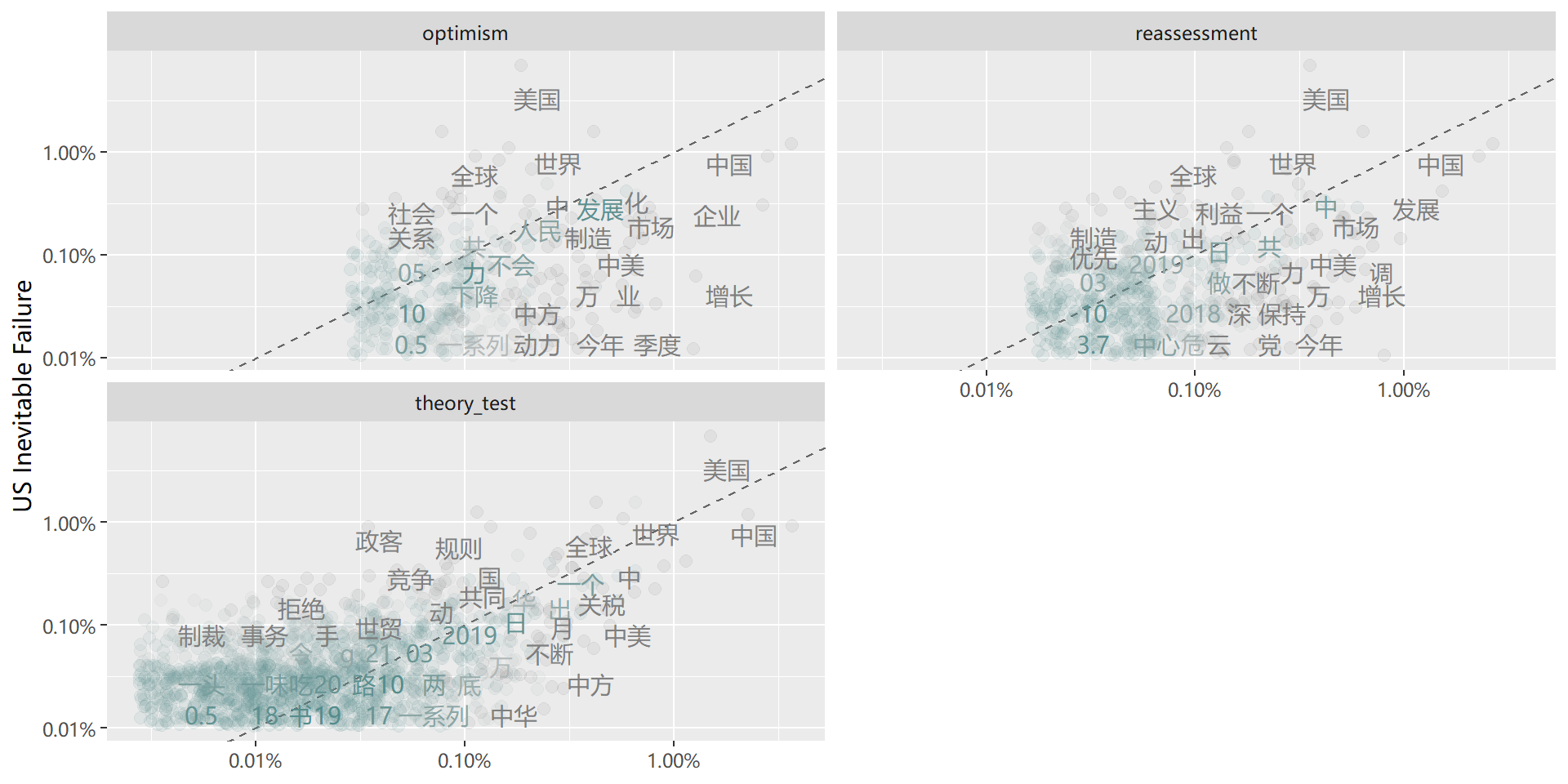
Frequency Correlations

frequency <- df_token |>
  count(phase, word) |>
  group_by(phase) |>
  mutate(proportion = n / sum(n)) |>
  select(-n) |>
  spread(phase, proportion) |>
  gather(phase, proportion, optimism:theory_test)

library(scales)

# expect a warning about rows with missing values being removed
ggplot(
  frequency,
  aes(x = proportion, y = `US_fail`, color = abs(`US_fail` - proportion))
) +
  geom_abline(color = "gray40", lty = 2) +
  geom_jitter(alpha = 0.1, size = 2.5, width = 0.3, height = 0.3) +
  geom_text(
    aes(label = word),
    check_overlap = TRUE,
    vjust = 1.5,
    family = cjk_font
  ) +
  scale_x_log10(labels = percent_format()) +
  scale_y_log10(labels = percent_format()) +
  scale_color_gradient(
    limits = c(0, 0.001),
    low = "darkslategray4",
    high = "gray75"
  ) +
  facet_wrap(~phase, ncol = 2) +
  theme(legend.position = "none") +
  labs(y = "US Inevitable Failure", x = NULL)

x = proportion, y = US_fail

proportion = n / sum(n)

Keyword analysis

Keywords for articles published on 2019-05-07

extractor_keyword <- worker("simhash", topn = 5)

simhash(
  df_zhongsheng$content[df_zhongsheng$time == "2019-05-07"],
  extractor_keyword
)

$simhash
[1] "4937328317770165287"

$keyword
 101.845  62.3717   58.696  57.5996  53.6127 
  "增长"   "韧性"    "GDP" "一季度"   "经济" 

Keywords for articles published on 2019-05-30

simhash(
  df_zhongsheng$content[df_zhongsheng$time == "2019-05-30"],
  extractor_keyword
)

$simhash
[1] "9551059633200593385"

$keyword
99.7583 56.3389 37.4295 35.7857 34.9402 
 "美国"  "政客"  "别国"  "国际"  "世界" 

Similarity analysis

Measuring the distance between texts

Hamming distance: the distance between two strings of equal length is the number of positions at which the corresponding symbols are different.

e.g., H(100→011) = 3; H(010→111) = 2.

It measures the minimum number of substitutions required to change one string into the other, or the minimum number of errors that could have transformed one string into the other.

Application

05-30 vs. 05-22

distance(
  df_zhongsheng$content[df_zhongsheng$time == "2019-05-30"],
  df_zhongsheng$content[df_zhongsheng$time == "2019-05-22"],
  extractor_keyword
)

$distance
[1] 30

$lhs
99.7583 56.3389 37.4295 35.7857 34.9402 
 "美国"  "政客"  "别国"  "国际"  "世界" 

$rhs
171.456 135.966 123.366 114.446 93.1847 
 "磋商"  "美方"  "中方"  "背弃"  "倒退" 

05-30 vs. 05-23

distance(
  df_zhongsheng$content[df_zhongsheng$time == "2019-05-30"],
  df_zhongsheng$content[df_zhongsheng$time == "2019-05-23"][1],
  extractor_keyword
)

$distance
[1] 18

$lhs
99.7583 56.3389 37.4295 35.7857 34.9402 
 "美国"  "政客"  "别国"  "国际"  "世界" 

$rhs
   137.594    91.4451    63.4508    53.6785    37.6035 
    "规则"     "美国"     "美方"     "国际" "世贸组织" 

Beyond “Bag of Words”

Bring the context back

• Analysis of function words (stopwords, parts of speech)
• Neighbor words: Markov Model of Order N
  • Unigram: 清华 大学 政治 系
  • Bigram: 清华大学 政治系/清华 大学政治 系
  • Trigram: 清华大学政治 系/清华 大学政治系

Frequency to Weighted Frequency

Cons of DTM

1. Not distinguish important words
2. Over-emphasize common words
3. Under-emphasize rare words

Solution: Word weights: e.g., term frequency-inverse document frequency (TF-IDF)

Word Weight

• Pros:
  1. Identify important words
  2. Reduce the weight of common words
  3. Improve the performance of machine learning models

• Cons:
  1. Assume independence of terms (same as DTM)
  2. Give high weight to words that are very rare in the corpus but appear a few times in a particular document
  3. Sensitive to the size and diversity of the corpus

Word embedding:

Words’ meanings depend not just on immediate neighbors

The term “embedding” comes from the neural network literature, in which an “embedding layer” is an input function that efficiently compresses high-dimensional data down to a low-dimensional dense representation for input to subsequent neural network layers.

• The embedding model GloVe (“Global Vectors”) by Pennington et al. (2014) is explicitly designed to construct word vectors encoding local co-occurrence.
• An equally influential word embedding model is Word2Vec (Bengio et al. 2000), which treats each instance of a word and its context as a separate prediction problem that word vectors are chosen to solve.

Topic modeling

LSA, NMF, and LDA can also be viewed as producing word embeddings. In particular, the (V × K) matrix B from (2) contains a series of row vectors corresponding to each term in the vocabulary (see also Levy and Goldberg 2014). Those vectors contain information about word co-occurrence at the document level, rather than within a local context.

Attention Function

Word embedding weights all the words equally in the context🤦‍♂️

“Attention is all you need” (Vaswani et al. 2017)

As a leading firm in the [MASK] sector, we hire highly skilled software engineers.
As a leading firm in the [MASK] sector, we hire highly skilled petroleum engineers.

What should be filled into the “[MASK]”? How do you figure it out?

As a leading firm in the [information technology] sector, we hire highly skilled software engineers.

As a leading firm in the [energy] sector, we hire highly skilled petroleum engineers.

Word Sequence

Self-attention function

Take as input a sequence of initial token embeddings and outputs a sequence of new token embeddings that allow the initial embeddings to interact.

• Massive neural networks composed of stacked attention and feed-forward neural network layers can be efficiently parallelized for training using specialized processors.
  • A.k.a., the Transformer
• Common transformer models
  • BERT
    • RoBERTa, PALM
  • The GPT family

Do LLMs make this obsolete?

Not at all—and not by belittling them.

Zero-shot ChatGPT beat crowd workers by ~25 points on stance and relevance labeling, at under 3¢ per label (Gilardi et al. 2023); on some tasks it even tops trained experts (Törnberg 2025).

So can an LLM label text? Often yes. The real question is: can you trust it?

Four cautions

• Uneven
• Biased stats
• LLM hacking
• Non-English

Across 27 replicated studies, GPT-4’s accuracy swung wildly—on some tasks precision or recall fell below 0.5, no better than a coin flip (Pangakis et al. 2023).

Even at 90% labeling accuracy, feeding labels straight into a regression yields biased coefficients and invalid intervals. Correcting it needs a small human “gold standard” plus classic inference (Egami et al. 2024).

Swapping the model or rewording a prompt flipped about one-third of conclusions in real replications; closed models also update silently (Baumann et al. 2025; Ollion et al. 2024).

Training data is English-dominated, and its biases are inherited (Bender et al. 2021). On fine-grained tasks a small fine-tuned model can beat zero-shot GPT-4 by 10–25 points (Bucher and Martini 2024).

Why classic methods still matter

1. Validation bedrock
2. Interpretability
3. Replicability

4. Resource efficiency
5. Theoretical grounding
6. Methodological bridge

The tools that “replace” the classics are exactly the classics you need to trust them.

The emerging workflow

1. LLM labels a subset
2. Train a lightweight local classifier
3. Validate against a human gold standard
4. Deploy to the full corpus

“Start small, start open, validate first.”

(Stoltz et al. 2026)

Wrap it up

• Principles
  1. All models are wrong
  2. Aim to assist humans
  3. No best method
  4. Validation, validation, validation
• Levels of analysis
  • Description
  • Classification
  • Semantics

• Procedure
  • Preprocessing
    • Segmentation
    • Tokenization
  • Frequency analysis
    • Frequency, dynamics, correlation
    • Keyword
  • Similarity analysis
  • Semantic analysis
    • Word embedding, sequence
      • Topic modeling

Thank you

  sammo3182

  yuehu@tsinghua.edu.cn

  https://www.drhuyue.site

References

Baumann, Joachim, Paul Röttger, Aleksandra Urman, et al. 2025. “Large Language Model Hacking: Quantifying the Hidden Risks of Using LLMs for Text Annotation.” arXiv Preprint arXiv:2509.08825, ahead of print. https://doi.org/10.48550/arXiv.2509.08825.

Bender, Emily M., Timnit Gebru, Angelina McMillan-Major, and Shmargaret Shmitchell. 2021. “On the Dangers of Stochastic Parrots: Can Language Models Be Too Big? 🦜.” (New York, NY, USA), FAccT ’21, March 1, 610–23. https://doi.org/10.1145/3442188.3445922.

Bengio, Yoshua, Réjean Ducharme, and Pascal Vincent. 2000. “A neural probabilistic language model.” Advances in Neural Information Processing Systems 13.

Benoit, Kenneth, Drew Conway, Benjamin E. Lauderdale, Michael Laver, and Slava Mikhaylov. 2016. “Crowd-Sourced Text Analysis: Reproducible and Agile Production of Political Data.” American Political Science Review 110 (2): 278–95. https://doi.org/10.1017/S0003055416000058.

Biber, Douglas. 1993. “Representativeness in Corpus Design.” Literary and Linguistic Computing 8 (4): 243–57. https://doi.org/10.1093/llc/8.4.243.

Black, Ryan C., Sarah A. Treul, Timothy R. Johnson, and Jerry Goldman. 2011. “Emotions, Oral Arguments, and Supreme Court Decision Making.” The Journal of Politics 73 (2): 572–81. https://doi.org/10.1017/s002238161100003x.

Bucher, Martin Juan José, and Marco Martini. 2024. “Fine-Tuned ‘Small’ LLMs (Still) Significantly Outperform Zero-Shot Generative AI Models in Text Classification.” arXiv Preprint arXiv:2406.08660, ahead of print. https://doi.org/10.48550/arXiv.2406.08660.

Coase, R. H. 1960. “The Problem of Social Cost.” The Journal of Law & Economics 56 (4): 837–77. https://doi.org/10.1086/674872.

Dietrich, Bryce J., Matthew Hayes, and Diana Z. O’Brien. 2019. “Pitch Perfect: Vocal Pitch and the Emotional Intensity of Congressional Speech.” American Political Science Review, Forthcoming.

Egami, Naoki, Musashi Hinck, Brandon M. Stewart, and Hanying Wei. 2024. “Using Imperfect Surrogates for Downstream Inference: Design-Based Supervised Learning for Social Science Applications of Large Language Models.” Pre-published January 14. https://doi.org/10.48550/arXiv.2306.04746.

Friedman, Milton, and Anna Jacobson Schwartz. 2008. A Monetary History of the United States, 1867-1960. Princeton University Press. https://books.google.com?id=Q7J_EUM3RfoC.

Gilardi, Fabrizio, Meysam Alizadeh, and Maël Kubli. 2023. “ChatGPT Outperforms Crowd Workers for Text-Annotation Tasks.” Proceedings of the National Academy of Sciences 120 (30): e2305016120. https://doi.org/10.1073/pnas.2305016120.

Grimmer, Justin. 2010. “A Bayesian Hierarchical Topic Model for Political Texts: Measuring Expressed Agendas in Senate Press Releases.” Political Analysis 18 (1): 1–35. https://doi.org/10.1093/pan/mpp034.

Grimmer, Justin, Margaret E. Roberts, and Brandon M. Stewart. 2022. Text as Data: A New Framework for Machine Learning and the Social Sciences. Princeton University Press. https://books.google.com?id=dL40EAAAQBAJ.

Grimmer, Justin, and Brandon M. Stewart. 2013. “Text as Data: The Promise and Pitfalls of Automatic Content Analysis Methods for Political Texts.” Political Analysis 21 (3): 267–97.

Lasswell, Harold D. 1927. “The Theory of Political Propaganda.” American Political Science Review 21 (03): 627–31.

Liu, Amy H. 2022. “Pronoun Usage as a Measure of Power Personalization: A General Theory with Evidence from the Chinese-Speaking World.” British Journal of Political Science 52 (3, 3): 1258–75. https://doi.org/10.1017/S0007123421000181.

Ollion, Étienne, Rubing Shen, Ana Macanovic, and Arnault Chatelain. 2024. “The Dangers of Using Proprietary LLMs for Research.” Nature Machine Intelligence 6 (1): 4–5. https://doi.org/10.1038/s42256-023-00783-6.

Pangakis, Nicholas, Samuel Wolken, and Neil Fasching. 2023. “Automated Annotation with Generative AI Requires Validation.” arXiv Preprint arXiv:2306.00176, ahead of print. https://doi.org/10.48550/arXiv.2306.00176.

Pennebaker, James W. 2017. “Mind Mapping: Using Everyday Language to Explore Social & Psychological Processes.” Procedia Computer Science, Data analytics summit II; structuring the UNSTRUCTURED: The missing element of analytics, 14-16 december 2015, harrisburg, USA, vol. 118 (January): 100–107. https://doi.org/10.1016/j.procs.2017.11.150.

Pennington, Jeffrey, Richard Socher, and Christopher Manning. 2014. “GloVe: Global Vectors for Word Representation.” Proceedings of the 2014 Conference on Empirical Methods in Natural Language Processing (EMNLP) (Doha, Qatar), October, 1532–43. https://doi.org/10.3115/v1/D14-1162.

Stoltz, Dustin S., Marshall A. Taylor, and Sanuj Kumar. 2026. “Selecting Language Models for Social Science: Start Small, Start Open, and Validate.” arXiv Preprint arXiv:2601.10926, ahead of print. https://doi.org/10.48550/arXiv.2601.10926.

Stone, Philip J., Robert F. Bales, J. Zvi Namenwirth, and Daniel M. Ogilvie. 1962. “The General Inquirer: A Computer System for Content Analysis and Retrieval Based on the Sentence as a Unit of Information.” Behavioral Science 7 (4): 484–98. https://doi.org/10.1002/bs.3830070412.

Su, Yu-Sung, Yanqin Ruan, Siyu Sun, and Yu-Tzung Chang. 2020. “A Pattern Recognition Framework for Detecting Changes in Chinese Internet Management System.” Journal of Social Computing 1 (1): 28–39. https://doi.org/10.23919/JSC.2020.0004.

Törnberg, Petter. 2025. “Large Language Models Outperform Expert Coders and Supervised Classifiers at Annotating Political Social Media Messages.” Social Science Computer Review 43 (6): 1181–95. https://doi.org/10.1177/08944393241286471.

Vaswani, Ashish, Noam Shazeer, Niki Parmar, et al. 2017. “Attention Is All You Need.” Advances in Neural Information Processing Systems 30.

Zhang, Han, and Jennifer Pan. 2019. “CASM: A Deep-Learning Approach for Identifying Collective Action Events with Text and Image Data from Social Media.” Sociological Methodology 49 (1): 1–57. https://doi.org/10.1177/0081175019860244.

Zipf, George Kingsley. (1949) 2016. Human Behavior and the Principle of Least Effort: An Introduction to Human Ecology. Addison-Wesley Press. Reprint, Ravenio Books.