Multiple Regression

Large N & Leeuwenhoek (70700173)

Yue Hu

Overview

Multiple regression
Goodness of fit: R²
Post-estimation inferences

1 Multiple regression

1.1 Expression

Terminology: Multivariate vs. Multiple

Population Regression Function (PRF, two explanatory variables): \[Y_i = \beta_0 + \beta_1X_{1i} + \beta_2X_{2i} + \epsilon_i.\]

According to CLRM: \(E[\epsilon_i|\boldsymbol{X}] = 0.\)

Sample Regression Function (SRF): \[Y_i = \hat\beta_0 + \hat\beta_1X_{1i} + \hat\beta_2X_{2i} + \hat \epsilon_i\]

1.2 How multiple regressions work intuitively

1.3 Meaning of β₁

To be BLUE,

\(min_{\hat\beta_0,\hat\beta_1,\hat\beta_2}\sum \hat \epsilon_i^2\)

\[\begin{align} \Rightarrow\frac{\partial \sum \hat \epsilon_i^2}{\partial\hat\beta_0}\to& \color{darkred}{0}\\ \frac{\partial \sum \hat \epsilon_i^2}{\partial\hat\beta_1}\to& \color{darkred}{0}\\ \frac{\partial \sum \hat \epsilon_i^2}{\partial\hat\beta_2}\to& \color{darkred}{0} \end{align}\]

When being BLUE:

\[\begin{align} \hat\beta_0 =& \bar Y - (\bar\beta_1X_{1i} + \bar\beta_2X_{2i}),\\ \hat\beta_1 =& \frac{[\sum(Y_i - \bar Y)(X_{1i} - \bar X_1)][\sum(X_{2i} - \bar X_2)^2-\sum(X_{1i} - \bar X_1)(X_{2i} - \bar X_2)]}{\sum(X_{1i} - \bar X_1)^2\sum(X_{2i} - \bar X_2)^2 - [\sum(X_{1i} - \bar X_1)(X_{2i} - \bar X_2)]^2}\\ =& \frac{\sum\hat r_{1i}(Y_i - \bar Y)}{\hat r_{1i}^2}, \end{align}\] where the \(\hat r_{1i}\) are the errors from the regression of \(X_{1i}\) on \(X_{2i}\) (i.e., \(X_{1i} = \hat\delta_0 + \hat\delta_1X_{2i} + \hat r_{1i}\)), the proportion that \(X_2\)cannot explain.

\(\hat\sigma^2 = \frac{\sum\hat \epsilon_i^2}{n - 3}.\)

Interpretation

Every unit change in X₁ leads to β₁ changes in Y on average, ceteris paribus/holding everything else constant.

Constant how? Sufficient or necessary condition of the variance of Y?

2 Goodness of Fit

2.1 R²: Multiple Coefficient of Determination

\[\begin{align} Y_i =& \hat Y_i + \hat \epsilon_i;\\ Y_i - \bar Y =& \hat Y_i - \bar Y + \hat \epsilon_i;\\ \Rightarrow (Y_i - \bar Y)^2 =& (\hat Y_i - \bar Y + \hat \epsilon_i)^2,\\ =& (\hat Y_i - \bar Y)^2 + \hat \epsilon_i^2 +, 2\hat\epsilon_i(\hat Y_i - \bar Y).\\ \text{Sum up, } \Rightarrow \sum(Y_i - \bar Y)^2 =& \sum(\hat Y_i - \bar Y)^2 + \sum\hat\epsilon_i^2.\\ SST =& SSR + SSE;\\ 1 =& \frac{SSR}{SST} + \frac{SSE}{SST}.\\ \text{In which, } R^2 =& \frac{\sum(\hat{Y} - \bar Y)^2}{\sum(Y - \bar Y)^2} = \frac{SSR}{SST} = \frac{\sum(\hat Y_i - \bar Y)^2}{SST},\\ =& \frac{\sum[\hat\beta_0 + (\hat\beta_1X_1 +\cdots +\hat\beta_nX_n) - \bar Y]^2}{SST}. \end{align}\]

2.2 Why Is R² Bad?

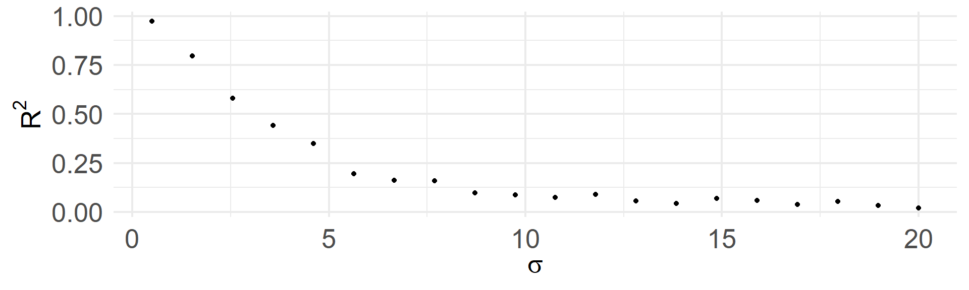
Reason 1: Can be very low for a correct model

\[\begin{align} R^2 =& \frac{\sum(\hat Y_i - \bar Y)^2}{SST}, \\ =& \frac{\sum[(Y_i - \color{darkred}{\epsilon_i}) - \bar Y]^2}{SST}. \end{align}\]

When the residual (thus σ, estimated by ε_i in a sample) is large enough, R² could approach a very low score towards zero.

2.3 Why Is R² Bad?

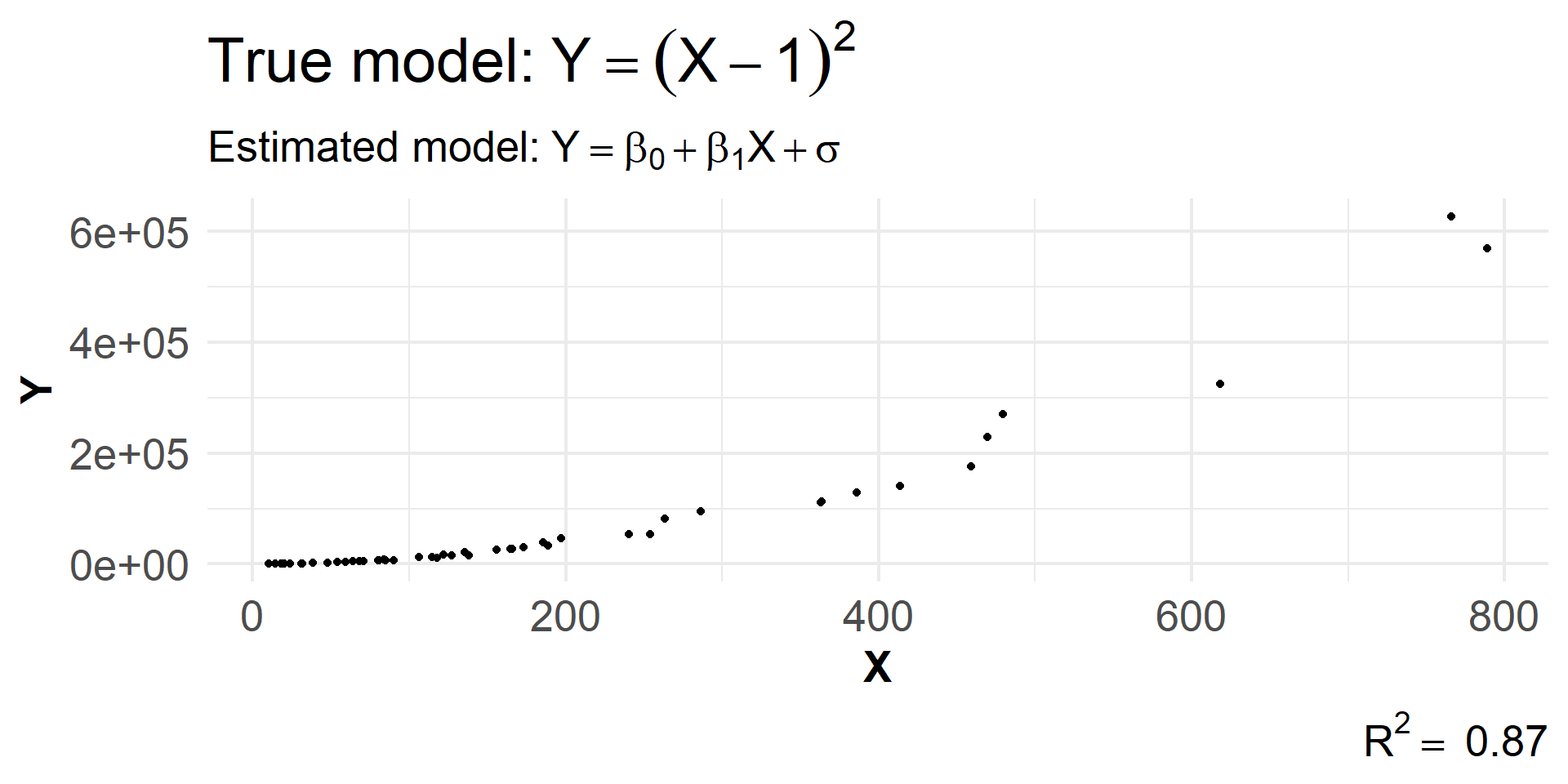
Reason 2: Can be very high for a misspecified model

2.4 Why Is R² Bad?

Reason 3: Can be very high for a redundant model

\[R^2 = \frac{\sum(\hat Y_i - \bar Y)^2}{SST} = \frac{\sum[\hat\beta_0 + (\hat\beta_1X_1 +\cdots +\hat\beta_nX_n) - \bar Y]^2}{SST}.\]

Therefore, the more Xs are added, the larger SSR (and thus R²) is, a.k.a., the “trash-can” model.

Revised statistics:

\[\text{Adj. } R^2 = 1 - (1 - R^2)\frac{n - 1}{n - k - 1}.\]

2.5 So, is Adj. R² good?

\[\text{Adj.} R^2 = 1 - (1 - R^2)\frac{n - 1}{n - k - 1}.\]

Adjusted

X booming

Not adjusted

Goodness of fit;
Predictive error;
Model comparison;
X’s explanatory power.

When can R² be useful then?

3 Post-Estimation Inferences

3.1 Predicted Value

Goal

Forecast
Interpretation:
- How is the model close to the reality?
- What extent of substantive changes can Xs make?

Approach

Expected value (average) of \(\hat Y\)
A one-time draw of \(\hat Y\)
Hypothesis testing

3.2 Forecasting: Expected Value

Let X₀ be the values of interest, and then calculate the \(\hat{Y}\):

\[\begin{align} E(\hat Y_0|X_0) =& E(\hat Y_0|X = X_0) = \boldsymbol{X_0\beta}\\ var(\hat Y_0|X_0) =& var(\hat\beta_0) + var(\hat\beta_1)X_0^2 + 2cov(\hat\beta_0, \hat\beta_1)X_0\\ =& \sigma^2[\frac{1}{n} + \frac{(X_0 - \bar X)^2}{\sum(X_i - \bar X)^2}]. \end{align}\]

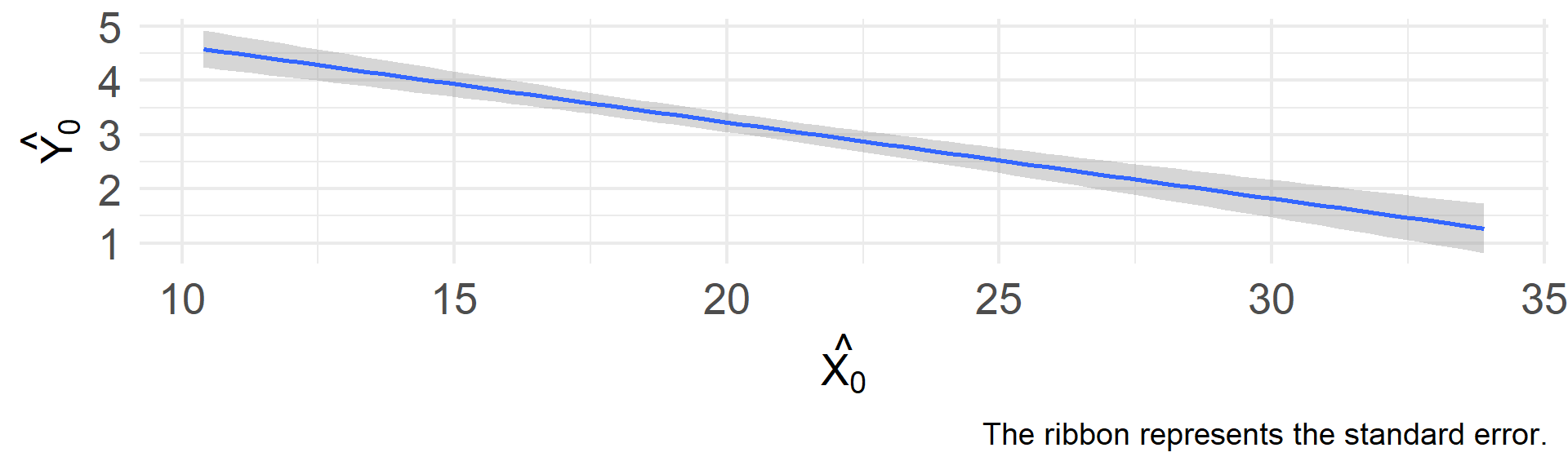
Why is the ribbon wider at the two ends?

3.3 Forcasting: Single-Point Forecast

\[\begin{align} \hat Y_0 =& \hat\beta_0 + \hat\beta_1X_0 + \hat u\\ var(\hat Y_0|X_0) =& \sigma^2[\color{darkred}{1} + \frac{1}{n} + \frac{(X_0 - \bar X)^2}{\sum(X_i - \bar X)^2}]. \end{align}\]

There is an extra error term to account for. In other words, single prediction is more uncertain than the average prediction.

3.4 Hypothesis Test: Coefficient and variance

Let α = 0.05.

1. On the coefficient

Hypothesis:

\[\begin{align} H_0: \beta =& \beta^*;\\ H_1: \beta \neq& \beta^*. \end{align}\]

Statistics:

\[\frac{\hat\beta - \beta^*}{\sqrt{\frac{\hat\sigma^2}{\sum(X_i - \bar X)^2}}}\sim t_{n-k}.\]

2. On the variance

Hypothesis:

\[\begin{align} H_0: \sigma =& \sigma^*;\\ H_1: \sigma \neq& \sigma^*. \end{align}\]

Statistics:

\[(n - k)\frac{\hat\sigma^2}{\sigma^2}\sim\chi^2.\]

3. Model structure: Restricted Model

Let’s set α = 0.05, \(H_0: \beta_1 + 2\beta_2 = 3\Rightarrow \beta_1 = 3 - 2\beta_2; H_1: \beta_1 + 2\beta_2 \neq 3.\)

Then,

\[\begin{align} Y =& \beta_0 + \beta_1X_1 + \beta_2X_2 + u, \text{(unrestricted)},\\ =& \beta_0 + 3X_1 + \beta_2(X_2 - 2X_1) + u;\\ \Leftrightarrow Y - 3X_1 =& \beta_0 + \beta_2(X_2 - 2X_1) + u;\\ Y^* =& \beta_0' + \beta_2'Z + u, \text{(restricted)}, \end{align}\] where \(Y^*=Y - 3X_1; Z = X_2 - 2X_1.\)

The test is thus transformed to \(H_0: \beta_2' = \beta_2; \beta_0' = \beta_0\).

Statistics:

\[\frac{\frac{SSR_R - SSR_U}{\Delta k}}{\frac{SSR_U}{n - k_U - 1}} = \frac{\frac{R_U^2 - R_R^2}{\Delta k}}{\frac{1 - R_U^2}{n - k_U - 1}}\sim F_{\Delta k, n - k - 1}\]

Important

If the hypothesis is rejected, the unrestricted model is better.

3.5 “When” to use OLS

3.6 Take-home point

Appendix: Latin phrases

Common Latin Phrases

a fortiori: Not even saying.
ad hoc: To this, immediate purpose.
ibid.: “ibidem,” in the same place.
ceteris paribus: with other conditions - remaining the same.
c.f.: “confer,” compare
e.g.: “exempli gratia,” for the sake of - example.
etc.: “et cetera,” and the rest.
i.e.: “id est,” that is.
n.b./NB: “nota bene,” note well.
per se: By/of/for/in itself.
QED: \(\blacksquare\) “quod erat demonstrandum,” that which was to have been shown.

Appendix

Stretch

Meditation

Multiple Regression

Overview

1 Multiple regression

1.1 Expression

1.2 How multiple regressions work intuitively

1.3 Meaning of β1

2 Goodness of Fit

2.1 R2: Multiple Coefficient of Determination

2.2 Why Is R2 Bad?

2.3 Why Is R2 Bad?

2.4 Why Is R2 Bad?

2.5 So, is Adj. R2 good?

3 Post-Estimation Inferences

3.1 Predicted Value

3.2 Forecasting: Expected Value

3.3 Forcasting: Single-Point Forecast

3.4 Hypothesis Test: Coefficient and variance

3.5 “When” to use OLS

3.6 Take-home point

Appendix: Latin phrases

Common Latin Phrases

Appendix

Stretch

Meditation

1.3 Meaning of β₁

2.1 R²: Multiple Coefficient of Determination

2.2 Why Is R² Bad?

2.3 Why Is R² Bad?

2.4 Why Is R² Bad?

2.5 So, is Adj. R² good?