Association Analysis

Large N & Leeuwenhoek (70700173)

Yue Hu

Overview

• Linear correlation
• Monotonic correlation
• Non-monotonic correlation

1 Linear Correlation

1.1 Etymoloy

 

 

1.2 Covariance

When one (X) changes, how much does the other (Y) respond?

Remember Variance?

\[\begin{align} \sigma^2_X =& \sum(X - \mu_X)^2p(X),\\ =& \sum(X - \mu_X)(X - \mu_X)p(X, X); \end{align}\]

\[\sigma_{X, Y} = \sum(X - \mu_X)\color{red}{(Y - \mu_Y)}p(X, \color{red}{Y}).\]

Covariance is literally the co-variance.

1.3 Correlation

When one (X) changes, how much % does the other (Y) respond?

1. Interpretability: Correlation is easier to interpret due to its standardization, while covariance values are often more complex to interpret due to their dependence on the units of the variables.
2. Scale: Covariance can take on any value, depending on the scale of the variables, while correlation always ranges from -1 to 1.
3. Standardization: Correlation is derived from covariance by dividing by the standard deviations of the variables, which standardizes the value.

Common Types:

• Karl Pearson’s r (Linear);
• Charles Spearman’s ρ (Monotonic);
• Maurice Kendall’s τ (Monotonic).

1.4 Pearson’s r

Assumptions

1. Continuous data
   
2. Linear Relationship (one-on-one)

For a population

\[\rho_{X,Y} = \frac{\sum(X - \mu_X)(Y - \mu_Y)p(x,y)}{\sqrt{\sum(X - \mu_X)^2p(X)}\sqrt{\sum(Y - \mu_Y)^2p(Y)}} = \frac{\sigma_{X, Y}}{\sigma_X\sigma_Y}.\]

For a sample

\[r_{XY}=\frac{\sum_{i=1}^n (x_i-\bar{x})(y_i-\bar{y})}{\sqrt{\sum_{i=1}^n(x_i-\bar{x})^2}\sqrt{\sum_{i=1}^n(y_i-\bar{y})^2}}.\]

• Karl Pearson was an English mathematician and biostatistician.
  • Establishing the discipline of mathematical statistics.
  • Founded the world’s first university statistics department at University College, London in 1911
  • Proponent of social Darwinism, eugenics and scientific racism.

Multiple regressions: \(partial\ r = \frac{b/SE}{\sqrt{(b/SE)^2 + (n - k -1)}}\), a.k.a., partial correlation.

1.5 Properties

1. ρ∈ [-1, 1], 0 independent.
2. Greater value indicates stronger linear relationship.
3. Parametric test¹
4. Not robust to skewed data and outliers.

Limitation

1. Which means assuming normal distribution, linearity, and homoscedasticity.

2 Monotonic Correlation

2.1 Ranking

Raw

x	y
26	95
18	35
12	14
21	30
15	25
20	45
17	20
22	60

→ Ordered

x	y
12	14
15	25
17	20
18	35
20	45
21	30
22	60
26	95

→ Ranked

x	x_rank	y	y_rank
12	1	14	1
15	2	25	3
17	3	20	2
18	4	35	5
20	5	45	6
21	6	30	4
22	7	60	7
26	8	95	8

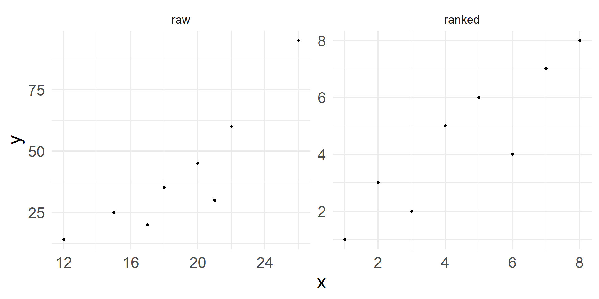
2.2 What does ranking change

2.3 Pairing

Define Pair

For any pair of observations x_i, y_i and x_j, y_j, i < j,

• Concordant pairs: x_i >x_j & y_i >y_j | x_i <x_j & y_i <y_j;

• Discordant pairs: x_i >x_j & y_i <y_j | x_i <x_j & y_i >y_j;

• Tied pairs: x_i = x_j & y_i = y_j

Solution for the monotonic yet non-linear variables

\[\text{Diff}_{quantity} \rightarrow \text{Diff}_{relation}.\]

tie on x or tie on y are also not concordant or discordant

2.4 Count the pairs

x_rank	y_rank	p1	p2	p3	p4	p5	p6	p7	c	d
1	1								0	0
2	3	+							1	0
3	2	+	-						1	1
4	5	+	+	+					3	0
5	6	+	+	+	+				4	0
6	4	+	+	+	-	-			3	2
7	7	+	+	+	+	+	+		6	0
8	8	+	+	+	+	+	+	+	7	0

2.5 Spearman’s rho: Ranking version of Pearson’s R

Assumptions

1. Continuous Ordinal/norminal;
2. Linear Monotonic

\(\rho _{\operatorname {rg} _{X},\operatorname {rg} _{Y}}={\frac {\operatorname {cov} (\operatorname {rg} _{X},\operatorname {rg} _{Y})}{\sigma _{\operatorname {rg} _{X}}\sigma _{\operatorname {rg} _{Y}}}},\) where \(rg\): the rank of the variables.

• When all n ranks are distinct integers (no tie): \(\rho_{s}={1-{\frac {6\sum d_{i}^{2}}{n(n^{2}-1)}}},\) where \(d_{i}=\operatorname {rg} (X_{i})-\operatorname {rg} (Y_{i}).\)
• Properties:
  • Independent, ρ = 0.
  • Calculation
    • Option 1: Fisher transformation (parametric), \(z={3(n_{c}-n_{d}) \over {\sqrt {n(n-1)(2n+5)/2}}}\)
    • Option 2: Permutation (nonparametric)

• Sir Maurice /MOR-iss/ George Kendall was a prominent British statistician.
  • The second chair of statistics at the London School of Economics, University of London

https://statistics.laerd.com/statistical-guides/spearmans-rank-order-correlation-statistical-guide.php

https://www.youtube.com/watch?v=XV_W1w4Nwoc

Still based on population parameters, so one can do significant test by \(z={3(n_{c}-n_{d}) \over {\sqrt {n(n-1)(2n+5)/2}}}\).

• Charles Edward Spearman was an English psychologist known for work in statistics, as a pioneer of factor analysis.
  • Models for human intelligence, including his theory that disparate cognitive test scores reflect a single General intelligence factor and coining the term g factor.

2.6 Tau: Robust Mnontonic Correlation

Kendall’s τ_A

\[\tau_{A}=\frac{n_c-n_d}{n_c+n_d}=\frac{n_c-n_d}{\binom{n}{2}},\]

• n_c: Number of concordant pairs
• n_d: Number of discordant pairs

In the previous example, n_c = Σc = 25, n_c = Σd = 3, t_x = u_j = 0.

\[\tau = \frac{25 - 3}{25 + 3} \approx 0.7857.\]

Remind problems: Ties? N(X) ≠ N(Y)?

2.7 Tau: Improved Versions

Kendall’s τ_B: Ties

\[\tau_{B}={\frac {n_{c}-n_{d}}{\sqrt {(n_{0}-n_{1})(n_{0}-n_{2})}}},\] where

\[\begin{aligned} n_{0}&=n(n-1)/2\\n_{1}&=\sum _{i}t_{i}(t_{i}-1)/2\\ n_{2}&=\sum _{j}u_{j}(u_{j}-1)/2\\n_{c}&={\text{Number of concordant pairs}}\\ n_{d}&={\text{Number of discordant pairs}}\\ t_{i}&={\text{Number of tied values in the }}i^{\text{th}}{\text{ group in X}}\\u_{j}&={\text{Number of tied values in the }}j^{\text{th}}{\text{ group of ties in Y}} \end{aligned}\]

Dealing with ties

Stuart’s τ_C: Diff scales

\[\tau _{C}={\frac {2(n_{c}-n_{d})}{n^{2}{\frac {(m-1)}{m}}}},\] where

\[\begin{aligned} n_{c}&={\text{Number of concordant pairs}},\\ n_{d}&={\text{Number of discordant pairs}},\\ m&=\min(r,c),\\ r&={\text{Number of rows}},\\ c&={\text{Number of columns}}. \end{aligned}\]

Dealing with retangle (nx != ny)

Ref: https://www.youtube.com/watch?v=Pm8KV5f3JM0

• Hypothesis testing: pure non-parametric
  • P-value is given through extensive simulation, such as Monte Carlo simulations

2.8 When to use which

type	estimate	statistic	p.value
r	0.8916	4.8223	0.0029
rho	0.9048	8.0000	0.0046
tau	0.7857	25.0000	0.0055

r vs. τ & ρ:

• r: Linear relationship;
• τ & ρ:
  • Monotonic relationship.
  • Ordinal variables

ρ vs. τ:

• τ is more robust than ρ;
• ρ has less cost than τ.

τ_A vs. τ_B: τ_B

What about categorical variables?

2.9 Correlations among Categorical/Nominal Variables: χ²

\[\chi^2 = \sum_i\sum_j \frac{(Observed - Expected)^2}{Expected} = \sum_{i,j}\frac{(n_{i,j}-\frac{n_{i\cdot}n_{\cdot j}}{n})^{2}}{\frac{n_{i\cdot}n_{\cdot j}}{n}}\]

E.g., The partisan distribution of American fathers and sons. Are they correlated?

Father/Son	D	R	I	Total
D	45	5	10	60
R	2	23	5	30
I	3	2	5	10
Total	50	30	20	100

\(H_0:\) Sons’ party ID has no relation with their fathers’; \(\pi_{ij} = \pi_i \pi_j, \forall\ i, j.\) (α = 0.05)

E(D_f, D_s) = 50/100 × 60/100 × 100 = 30.

\[\begin{align} \chi^2 =& \frac{(45 - 30)^2}{30} + \frac{(5 - 18)^2}{18} + \dots + \frac{(5 - 2)^2}{2}\\ \approx& 56.07, d.f.: (r - 1)(c - 1) = (3 - 1)^2 = 4. \end{align}\]

\(\chi^2_{critical} = \chi^2_{0.05, 4} =\) 11.1433< \(\chi^2_{observed}\). Thus, H₀ is rejected.

2.10 Adjustment of χ²

Why adjusting

1. When sample is too small and/or having too many missing data, the distribution might be different from \(\chi^2\)
2. When N gets large, \(\chi^2\) also increase (esp. over 100,000)

→ Φ and Cramer’s V

• \(\Phi = \sqrt{\frac{\chi^2}{n}}\in[0, 1]\)
  • 2×2 table
  • 0 means no association
  • 1 means perfect association

phi

• Cramer’s V
  • Beyond a 2*2 table (when \(\Phi\) > 1).
  • \(V = \sqrt{\frac{\chi^2}{n\times min_{r-1, c-1}}}\).

2.11 ANOVA: If detecting the difference is enough

Analysis of variance (ANOVA): A systematic way of variable comparison in the context of experiment.¹

Assumption

1. Y normally distributed in each group (Type I ↓)
2. Homogeneity of variance (Type I & II ↓)
3. Independence of cases (Type I ↓)
4. No large outliers (Type II ↓)
5. Large sample (Type I & II ↓)

When there are more than one treatment group, ANOVA is more useful to reduce the risk of Type I (“Hey grandpa, you are pregnant”).

1. Equivalent to t-test.

2.12 One-Way ANOVA

• \(\overline X\), sample mean; the grant mean \(\overline{\overline{X}} = \frac{\sum \overline{X_i}}{K}\), where K is column number.¹
• SST: Variance between the samples; SSE: Variance within the samples.²

Source	Sum Square	d.o.f.	Mean Square
Treat	\(SST = \sum n_i (\bar X_i - \overline{\overline{X}})^2\)	K - 1	MST = SST/(K - 1)
Error	\(SSE = \sum \sum (X_{ik} - \bar{X_i})^2\)	N - K	MSE = SSE/(N - K)
Total	\(SS = SST + SSE\)	N - 1

\[F_{\alpha, K-1, N-k} = \frac{MST}{MSE} = \frac{\text{Ratio of Explained Variance}}{\text{Ratio of Unexplained Variance}}.\]

1. ANOVA is usually used when \(K \in [2, 3]\); for larger K, often use MANOVA (rarely used in Poli Sci).

2. Χ² is adding-up of n square normals representing variances; F is the ratio of two χ²s. In other words, they are consistent with t-test and OLS.

2.13 Example

The following table shows the funding applications of six faculty members of Xavier Institution. Does mutants willingness of application relate to the funding type?

NS	ME	BJ
27	23	48
22	36	35
33	27	46
25	44	36
38	39	28
29	32	29

\(H_0: \mu_1 = \mu_2 = \mu_3,\)
\(H_1: \mu_1 \neq \mu_2 \neq \mu_3.\)

α = 0.05.

\[\begin{align} \bar X_{NS} &= 29; \bar X_{ME} = 33.5; \bar X_{BJ} = 37;\\ \bar{\bar{X}} &= (29 + 33.5 + 37)/3 \approx 33.17 \end{align}\]

2.14

\(H_0: \mu_1 = \mu_2 = \mu_3,\)
\(H_1: \mu_1 \neq \mu_2 \neq \mu_3.\)

α = 0.05.

\[\begin{align} \bar X_{NS} &= 29; \bar X_{ME} = 33.5; \\ \bar X_{BJ} &= 37;\\ \bar{\bar{X}} =& (29 + 33.5 + 37)/3 \approx 33.17 \end{align}\]

Then, \(SST = \sum 6\times (\bar X - \bar{\bar{X}}) = 193\); \(SSE = [(27 - 29)^2 + (22 - 29)^2 + \dots + (29 - 37)^2] = 819.5\).

Given K = 3, N = 18, \(F = \frac{193/(3 - 1)}{819.5/(18 - 3)} \approx 1.77\)

\(F_{0.05, 2, 15}\) = 4.7650483 \(F_obs\), so fail to reject \(H_0\)

Source	Sum Square	d.o.f.	Mean Square
Treat	\(SST = \sum n_i (\bar X_i - \bar{\bar{X}})^2\)	K - 1	MST = SST/(K - 1)
Error	\(SSE = \sum \sum (X_{ik} - \bar{X_i})^2\)	N - K	MSE = SSE/(N - K)
Total	\(SS = SST + SSE\)	N - 1	\(F_{\alpha, K-1, N-K} = MST/MSE\)

2.15 Two-Way ANOVA

• Randomized block design (i blocks, j groups)
  • Equivalent to matched sample in t-test¹

Source	Sum Square	d.o.freedom	Mean Square
Treat	\(SS_A: b\sum (\bar X_i - \bar{\bar{X}})^2\)	a - 1	MST_A = SS_A/(a - 1)
Block	\(SS_B: a\sum (\bar X_j - \bar{\bar{X}})^2\)	b - 1	MST_B = SS_B/(b - 1)
Error	\(SS_E: \sum^{ab} (X_{ij} - \bar{X_i} - \bar{X_j} + \bar{\bar{X}})^2\)	(a - 1)(b - 1)	\(MSE = \frac{SSE}{(a - 1)(b - 1)}\)
Total	\(SS: SS_A + SS_B + SS_E\)	ab - 1	\(F_{\alpha, a-1, b-1} = \frac{MST_{A or B}}{MSE}\)

1. Ranking version of ANOVA: Kruskal-Wallis test, Friedman test.

2.16 Example

Students’ final scores in three majors were recorded in the following table. Does the scores associate with majors?

Major	Poli Sci	Sociology	Psychology
A+	41	45	51
A	36	38	45
B+	27	33	31
B	32	29	35
C+	26	21	32
C	23	25	27

\(H_0: \mu_{PS} = \mu_{SO} = \mu_{PY},\)
\(H_1: \mu_{PS} \neq \mu_{SO} \neq \mu_{PY}.\)

α = 0.05.

\(\bar A_+ = 45.67; \bar A = 39.67; \bar B_+ = 30.33; \bar B = 32; \bar C_+ = 29.67; \bar C = 25.\)

\(\bar X_{PS} = 30.8; \bar X_{SO} = 33.5; \bar X_{PY} = 36.83, \bar{\bar{X}} = 33.72.\)

For factor A (major), \(SS_A = 6\times [(30.8 - 33.72)^2 + (33.5 - 33.72)^2 + (36.83 - 33.72)^2] = 109.48.\)

\(MSA = SS_A/(a - 1) = 109.48/(3 - 1).\)

For factor B (GPA), \(SS_B = 3\times [(45.67 - 33.72)^2 + \dots + (25 - 33.72)^2] = 854.94.\)

\(MSB = 854.94 / (6 - 1).\)

\(SST = \sum^a\sum^b(X_{ij} - \bar{\bar{X}})^2 = 1015.61; SSE = SST - SS_A - SS_B = 52.2\)

Then, \(F_{(3 - 1), (3 - 1)(6 -1)} = MS_A/MSE = \frac{109.5/(3 -1)}{52.2/(3 - 1)(6 - 1)}\) is 10.4 > critical F 5.4564, reject \(H_0\).

3 Beyond Monotonic

3.1 Complete the correlation census (Chatterjee 2021)

A solution: \(\xi\) correlation

Chatterjee, Sourav. 2021. “A New Coefficient of Correlation.” Journal of the American Statistical Association 116(536): 2009–22.

1. Linearity/monotoncity any functional correlation
2. As simple as the classical coefficients like Pearson’s correlation or Spearman’s correlation
3. Consistently estimates simple and interpretable measure of the degree of dependence between the variables (0, independent; 1 associated)

3.2 Property of \(\xi\)

Asymptotic estimate: As \(n\) goes to Infinity…

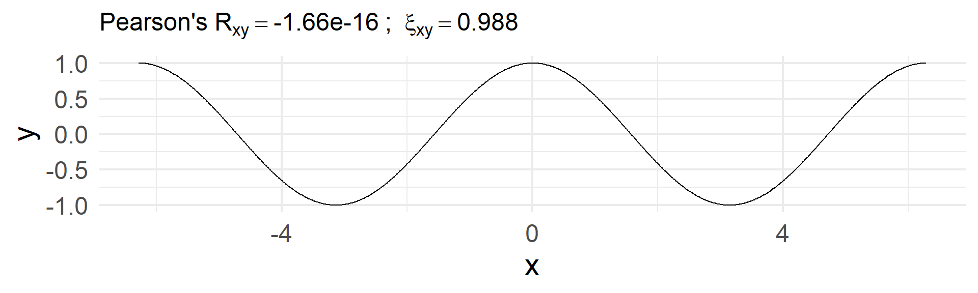
• If \(y\) is a function of \(x\), then \(\xi\) goes to 1 asymptotically as \(n\) (the number of data points, or the length of the vectors \(x\) and \(y\)) goes to infinity.
• If \(y\) and \(x\) are independent, then \(\xi\) goes to 0 asymptotically .
• No anti-correlation

3.3 Take-home point

3.4 Greek Letters

• β, “veta”
• γ, “hramma”
• δ/Δ “thzeita”
• ε
• θ
• λ “lamza”
• μ “mi”

• ρ “alorr”
• σ: “xigma”
• τ “tough”
• π “pi”
• ξ, “ksee”
• φ, “fi”
• χ, “he”
• ω/Ω, “omeha”

4 Appendix

4.1 Stretch

https://www.bilibili.com/video/BV1E54y1r76o/?buvid=Y045340D2FD9FA3A46419EEFE4578279ECBD&from_spmid=main.space-search.0.0&is_story_h5=false&mid=7RnjBONLRMus4FQZFBWD2g%3D%3D&p=2&plat_id=114&share_from=ugc&share_medium=iphone&share_plat=ios&share_session_id=79FE08C9-F2B1-4C18-A16C-B31179817B42&share_source=WEIXIN&share_tag=s_i&timestamp=1728732278&unique_k=skSWw7j&up_id=390316092&vd_source=f38aeefd0d38cecba9017eeee43e71c8

4.2 Meditation

松茸的世界：5分钟正念冥想-自信之心

https://www.xiaoyuzhoufm.com/episode/65b752ed0bef6c207457f51b?s=eyJ1IjogIjYwNDA1OGJiZTBmNWU3MjNiYmY3MjZiZSJ9

4.3 Ranking version of ANOVA

Analysis of variance-rank + Kruskal-Wallis test; + Friedman test.

4.4 One-Way Variance-Rank: Kruskal-Wallis Test

An extension of the two-sample Wilcoxon test

Procedure:

• Combine k samples and sorting
  • If the value are the same, use the average;
  • Let n_k as the size of the k sample, and n = ∑n_i, i ∈ {1, 2, …, k}.
• Calculate the rank sum of each sample, R_i
• \(H = \frac{12}{n(n + 1)}\sum^k_{i = 1}\frac{R^2_i}{n_i} - 3(n + 1) \sim \chi^2(k - 1).\)

4.5 Example

Botanists conducted an experiment of plant growth. The data records the results obtained under a control and two different treatment conditions (as measured by dried weight of plants).

group	count	mean	sd	median	IQR
ctrl	10	5.032	0.5830914	5.155	0.7425
trt1	10	4.661	0.7936757	4.550	0.6625
trt2	10	5.526	0.4425733	5.435	0.4675

kruskal.test(weight ~ group, data = PlantGrowth)

    Kruskal-Wallis rank sum test

data:  weight by group
Kruskal-Wallis chi-squared = 7.9882, df = 2, p-value = 0.01842

4.6 Two-Way Variance-Rank: Friedman Test

An extension of the sign test, and also a special case of Durbin test.

E.g., Person’s recovery score after taking four types of drugs. The type 1 is the placebo.

Rows: 20
Columns: 3
$ person <int> 1, 1, 1, 1, 2, 2, 2, 2, 3, 3, 3, 3, 4, 4, 4, 4, 5, 5, 5, 5
$ drug   <dbl> 1, 2, 3, 4, 1, 2, 3, 4, 1, 2, 3, 4, 1, 2, 3, 4, 1, 2, 3, 4
$ score  <dbl> 30, 28, 16, 34, 14, 18, 10, 22, 24, 20, 18, 30, 38, 34, 20, 44, 26, 28, …

friedman.test(y = df_drug$score,
              groups = df_drug$drug,
              blocks = df_drug$person)

    Friedman rank sum test

data:  df_drug$score, df_drug$drug and df_drug$person
Friedman chi-squared = 13.56, df = 3, p-value = 0.00357

⇒ Different type of drugs lead to different type of outcomes.

4.7 Association for Matched Samples: Ranking

Observation	Test 1	Test 2	Δ
1	X1	Y1	X1 - Y1
2	X2	Y2	X2 - Y2
3	X3	Y3	X3 - Y3

Goal: whether test 1 and test 2 yield identical results.

• +: X_i > Y_i;
• -: X_i < Y_i;
• =: X_i = Y_i;

Expectation: if test 1 and 2 are identically distributed, the probability of Δ to be + or - should follow the binomial distribution. That is, H₀: Pr(+) = Pr(-) = 0.5.

4.8 Sign Test

Observation	Test 1	Test 2	Δ	Sign
1	37	40	−3	−
2	72	73	−1	−
3	57	59	−2	−
4	44	43	1	+
5	43	51	−8	−
6	64	67	−3	−
7	55	61	−6	−
8	65	74	−9	−

H₀: Pr(+) = Pr(-) = 0.5;
H₁: Pr(+) < Pr(-).

α = 0.05

\[\begin{align} Pr(n_-\geq 7) =& Pr(n_- = 7) + Pr(n_- = 8)\\ =& {8 \choose 7}(0.5)^7(0.5)^1 + {8 \choose 8}(0.5)^8\\ =& 0.03125 + 0.0039 = 0.03516 < 0.05. \end{align}\]

4.9 Procedure of Sign Test

1. Calculate the Δ (or d);
2. Giving the sign accordign to d, if d = 0, ignore the observation;
3. Calculate n_- and n₊, n = n_- + n₊
4. Set H₀ and H₁, and α
5. Calculate Pr(+/-)
   • \(Pr(+) = \sum^{n_-}_{i = 0}Pr(n_+ + i)\);
   • \(Pr(-) = \sum^{n_+}_{j = 0}Pr(n_- + j)\);
6. Compare the Pr(+/-) with α.

Although claiming non-parametirc, many of them calculate the significance according to populational parameters.

Hint:

1. Work on matched and nonmatched samples.
2. It is essentially a binomial test (again, “non-parametric” test).

    Exact binomial test

data:  7 and 8
number of successes = 7, number of trials = 8, p-value = 0.03516
alternative hypothesis: true probability of success is greater than 0.5
95 percent confidence interval:
 0.5293206 1.0000000
sample estimates:
probability of success 
                 0.875 

4.10 Normal Approximation of Sign Test

(Often used when n > 10, why? Well…)

Using normal distribution to estimate sign tests:

μ = np = n/2; σ² = np(1 - p) = n/4.

\[Z = \frac{x' - \mu}{\sigma} = \frac{2x' - n}{\sqrt{n}},\] where x’= \[\begin{cases} x + 0.5, if x > \frac{n}{2}\\ x- 0.5, if x < \frac{n}{2} \end{cases}\]

¹

e.g., n = 8, then \(Pr(n_-\geq 7)\) ?

\[\begin{align} Z =& \frac{x' - \mu}{\sigma} = \frac{2x' - n}{\sqrt{n}},\\ =& \frac{2(7 - 0.5) - 8}{\sqrt{8}} = 1.77. \end{align}\]

Then, Pr(Z ≥ 1.77) ≈ 0.038 < 0.05.

1. ±0.5 approximate to a continuous variable as an expedient, a.k.a., normal approximation.

4.11 Advanced Version of Sign Test

Problems of sign test?

⇒ Wilcoxon signed-rank test

Sign test ony identify the sign but not the magnitude, insufficiently using the data.

1. Calculate the d and .red[|d|];
2. Sort these quantities, and record their rankings as R_i so that 0 < |d_R1| < |d_R2| <…< |d_Rn|.
3. Let sign function sgn(d) = 1 if d > 0, sgn(d) = -1, if d < 0, then calculate the signed-rank sum \(T = \sum^n_{i=1}sgn(d_i)R_i.\)
   • \(T^{+}=\sum _{d_{i}>0}R_{i},\)
   • \(T^{-}=\sum _{d_{i}<0}R_{i}.\)
4. Compare the Pr(T) with α.

Observation	Test 1	Test 2	Δ	Ranking
1	37	40	−3	4
2	72	73	−1	1
3	57	59	−2	3
4	44	43	1	1
5	43	51	−8	7
6	64	67	−3	4
7	55	61	−6	6
8	65	74	−9	8

wilcox.test(tb_sr$Test_1, tb_sr$Test_2, paired = TRUE)

Warning in wilcox.test.default(tb_sr$Test_1, tb_sr$Test_2, paired = TRUE): cannot
compute exact p-value with ties

    Wilcoxon signed rank test with continuity correction

data:  tb_sr$Test_1 and tb_sr$Test_2
V = 1.5, p-value = 0.02471
alternative hypothesis: true location shift is not equal to 0

• When tie happens, using Monte Carlo conditional p-value (coin::wilcox_test) to conduct outcomes .
• When n > 25, a normal approximation can be also conducted.

4.12 Ranking Test for Nonmatched Samples

Given samples S1 and S2,

• Rank-sum test
• Wald-Wolfowitz Runs Test

• Combining S1 and S2 and rank the pooled observations;
• Adding the ranking quantities (i.e., Rs in signed-rank test);
• Comparing the sums.

Meaning: Values of sorted S1 and S2 randomly occure?

Procedure:

1. Combine S1 and S2
2. Sorting the quantities
3. Giving those from S1 as 0 and those from S2 1 within their ranking order.
4. Testing whether the 0/1 occur stocastically.

When n₁ ≥ 20, n₂ ≥ 20, one can use normal approximation

Runs test means to test whether an item comes from population 1 and population 2 is random or not

4.13 Runs

Trial	1	2	3	4	5	6	7	8
A	9	22	65	34	17	4	31	28
B	58	53	26	11	52	51	8

⇓

4	8	9	11	17	22	26	28	31	34	51	52	53	58	64
0	1	0	1	0	0	1	0	0	0	1	1	1	1	0

4.14 Example

vec_runs1 <- rep(c(0,1), times = 5)
vec_runs2 <- rep(c(0,1), each = 5)
vec_runs3 <- c(1, 0, 0, 1, 1, 1, 1, 0, 0, 0)

vec_runs1 # nonrandom

 [1] 0 1 0 1 0 1 0 1 0 1

vec_runs2 # nonrandom

 [1] 0 0 0 0 0 1 1 1 1 1

vec_runs3 # random

 [1] 1 0 0 1 1 1 1 0 0 0

library(randtests)

runs.test(vec_runs1)

    Runs Test

data:  vec_runs1
statistic = 2.6833, runs = 10, n1 = 5, n2 = 5, n = 10, p-value = 0.00729
alternative hypothesis: nonrandomness

runs.test(vec_runs2)

    Runs Test

data:  vec_runs2
statistic = -2.6833, runs = 2, n1 = 5, n2 = 5, n = 10, p-value = 0.00729
alternative hypothesis: nonrandomness

runs.test(vec_runs3)

    Runs Test

data:  vec_runs3
statistic = -1.3416, runs = 4, n1 = 5, n2 = 5, n = 10, p-value = 0.1797
alternative hypothesis: nonrandomness