Confidence Intervals and Distribution Comparison

Large N & Leeuwenhoek (70700173)

Yue Hu

Overview

1. Sample properties
2. Confidence interval
3. Application

Connection with previous lectures

1. Still one single variable
2. Distribution in the last lecture is the distribution of a random variable
   • → the reference to calculate the confidence intervals
3. Also relating with prediction (“expectation”)

1 Sample property

1.1 Random Variable

• A random variable is a mathematical function that assigns numerical values to each possible outcome from a random experiment or process in the population.

  • Technically, a random (stochastic) variable is a type of variable in statistics whose possible values depend on the outcomes of a certain random phenomenon.

Different “variables”

• Variable in algebra: \(Y = log((\sqrt{X})^{\frac{1}{e}}) - 15.\)
• Variable in data analysis: “I asked about the respondents’ gender, age, and education.”

Not 1 map 1 or 1 map all, but there is a chance

Not fixed but may change

• Distribution for a random variable: The description of how likely a random variable takes one of its possible states.

1.2 Distribution and random variable

• Remember what’s the definition of a probability distribution?
  • The mathematical function that gives the probabilities of occurrence of different possible outcomes for an experiment.

Which is a function,
the random variable or the distribution?

• Both
  • Random variable: Outcomes → values.
  • Probability distribution: Probabilities → values.

Next step: Random variable (distribution) → population

1.3 Populaiton

• A random variable is a function that assigns numerical values to each possible outcome from a random process in the population.
• Population is the collection of all possible outcomes of a random variables
• The probability distribution is a function defining how these outcomes occur/exist in the population.

2024

• Official news is “略超 2:1”https://www.tsinghua.edu.cn/info/1182/113140.htm
• 网易：男女比例是2.42：1（https://m.163.com/dy/article/JAI5076G0549R6EJ.html?clickfrom=subscribe&spss=adap_pc）(which means about 29% are females)

1.4 Random Sample

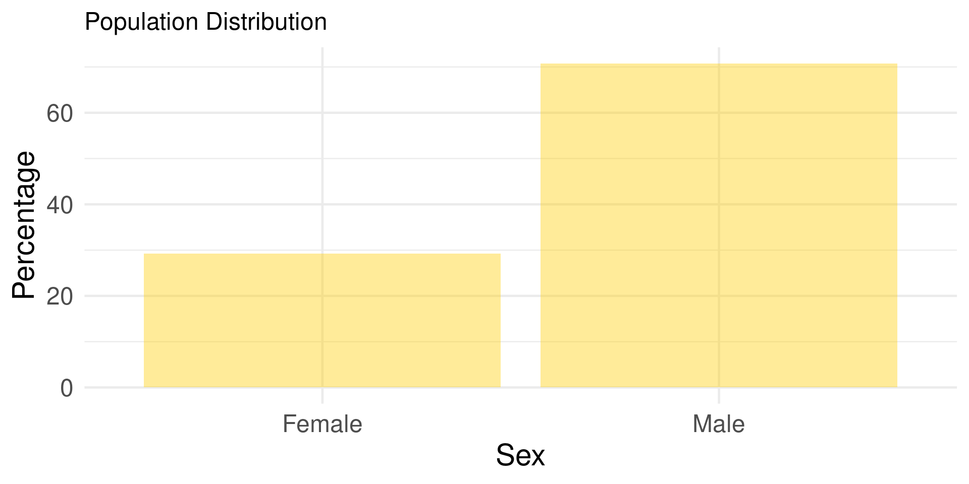
A sample: 2024 students in our class

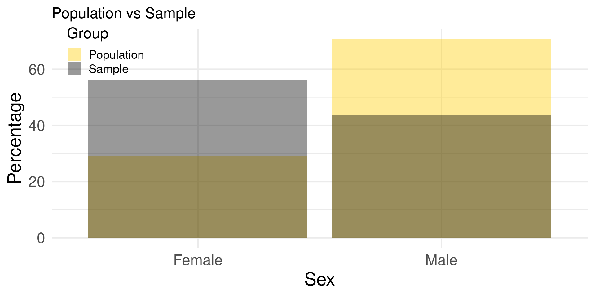
Is this a good sample?

1.5 A random sample

A subset of individuals or observations selected from a larger population in such a way that each observation has an equal probability of being chosen.

• Why is this good?
  • Random sample proerties
    • Finite ~
    • Large ~

1.6 Finite random sample properties

• Unbiasedness: Produce the right expectation on coverage, E(p) = π
  • Assuming independent and identical distribution (i.i.d)¹

• Unbiasedness: the expectation is the true value
  • Under the assumption that the random variables X1,X2,…,Xn are independently and identically distributed (i.i.d) with mean μ, each of the terms E(X1),E(X2),…,E(Xn) equals μ. Sampling with replacement
  • $ E({X}) = E((X_1 + X_2 + … + X_n)) = (E(X_1) + E(X_2) + … + E(X_n)) = (n) = . $
• How to achieve unbiasedness:
  1. Design: Randomization(prior), why? no confounders
  2. Post-dgp: weight(post), manually collect, 老将出马

• Efficiency: Smaller variance of an unbiased estimator²
  • \[\begin{align} Var(\bar{X}) =& \frac{\sigma^2}{n}, \\ =& Var(\frac{1}{n}(X_1 + X_2 + ... + X_n)), \\ =& \frac{1}{n^2} \cdot Var(X_1 + X_2 + ... + X_n) = \frac{1}{n^2} \cdot n\sigma^2. \end{align}\]
  • \(SE = \frac{\sigma}{\sqrt{n}}\), that is, how far \(\bar X\) disperse from μ.

• The median will generally be better than the mean if there are heavy tails, while the mean will be best with light tails.
• FSM: Flying Spaghetti Monster

How can you increase the efficiency?

1. W. or w.o., rep?

2. \(\text{Var}(aX) = a^2 \cdot \text{Var}(X).\)

1.7 Large random sample properties

• Convergence: \(p\lim_{n \to \infty}X_n = a, a\in R.\)

• When a sequence of random variables stabilizes to a certain probabilistic behavior as n → ∞ , the sequence is said to show stochastic convergence.
• Two Views of Convergence
  1. In probability: Values in the sequence eventually take a constant value (i.e. the limiting distribution is a point mass).
  2. In distribution: Values in the sequence continue to vary, but the variation eventually comes to follow an unchanging distribution (i.e. the limiting distribution is a well characterized distribution)

• Consistency:
  \(p\lim_{n \to \infty}\hat{\theta}_n = \theta.\)

An estimator q_n is consistent if the sequence q₁…q_n converges in probability to the true parameter value θ as sample size n grows to infinity

1.8 About Consistency

• Minimal requirement for estimators
• May perform badly in small samples

Only if a sequence of estimators is unbiased and converges to a value, then it is consistent, as it must converge to the true value.

• Does unbiasedness imply consistency?
  • How to estimate the expected height of our class?
• Does consistency imply unbiasedness?
  • \({1 \over n}\sum x_{i}+{1 \over n}\) consistent? unbiased?

• e.g., Let’s estimate the mean height of our class. To do so, we randomly draw a sample from the student population and measure their height. Then what estimator should we use? (Appendix C of Introductory Econometrics by Jeffrey Wooldridge)
  • Options: Both estimator are unbiased (😱!!!)
    1. The mean height of the sample;
    2. The height of the student we draw first.
  • E(X̄) = E(X₁) = μ;
  • Var(X1)=σ² forever; var(X̄) = σ²/n.

Say we want to estimate the mean of a population. While the most used estimator is the average of the sample, another possible estimator is simply the first number drawn from the sample. This estimator is unbiased, because E(X1)=μ due to the random sampling of the first number.

Yet the estimator is not consistent, because as the sample size increases, the variance of the estimator does not reduce to 0. Rather it stays constant, since Var(X1)=σ2 , which the population variance, again due to the random sampling. The additional information of an increasing sample size is simply not accounted for in this estimator.

• \({1 \over n}\sum x_{i}+{1 \over n}\) consistent? unbiased?
  • Consistent: As \(n\rightarrow \infty\), the estimator approaches the correct value, so it is consistent.
  • Biased: \(E({1 \over n}\sum x_{i}+{1 \over n}) = E({1 \over n}\sum x_{i})+E({1 \over n}) = \mu + {1 \over n}\neq \mu.\)

2 Confidence Interval

2.1 Learning the population from a sample

• X: a random sample from a probability distribution with parameter θ.

• Confidence interval (CI) for the parameter θ, with confidence level γ: An interval determined by random variables u(X) and v(X) with the property: \(Pr\{u(X)<\theta <v(X)\}\ =\ \gamma = 1 - \alpha, \quad \forall\theta.\)

• Human language: In a repeatedly sampling, the percentage of the samples that could contain θ

2.2 Calculated CI (Two-tailed)¹

• \(\bar X \pm Z_{\alpha/2}SE\)
  • α: 1 - Confident level;
  • Z-score: \(Z = \frac{X - \mu}{\sigma}\) Learned
• Proportion: \(\pi = P \pm Z_{\alpha/2}\sqrt{\frac{P(1 - P)}{n}}\)

s is the sample standard distribution, \(SE(\bar{X}) = \sqrt{\frac{s^2}{n}}\)

Interpretation

In 100 times sampling of …, there are … samples (… of the chance) that the CI could contain the true value.

How can you get smaller CI?

1. Large N
2. Large α
   • α = 0.05, Z = 1.959964
   • α = 0.1, Z = 1.6448536

1. Explained in the next lecture.

2.3 When N is not that large

Solution: A fatter-tailed distribution

• Small N, more probability to get dispersed result; more “uncommon” event can happen when the sample is smaller
  • t = (Φ / χ²)^(1/2)
• History:
  • First derived as a posterior distribution in 1876 by Helmert and Lüroth.
  • William Sealy Gosset, an English statistician, chemist and brewer, published in English language in Biometrika in 1908 using the pseudonym “student.” Fisher called it the “student distribution”

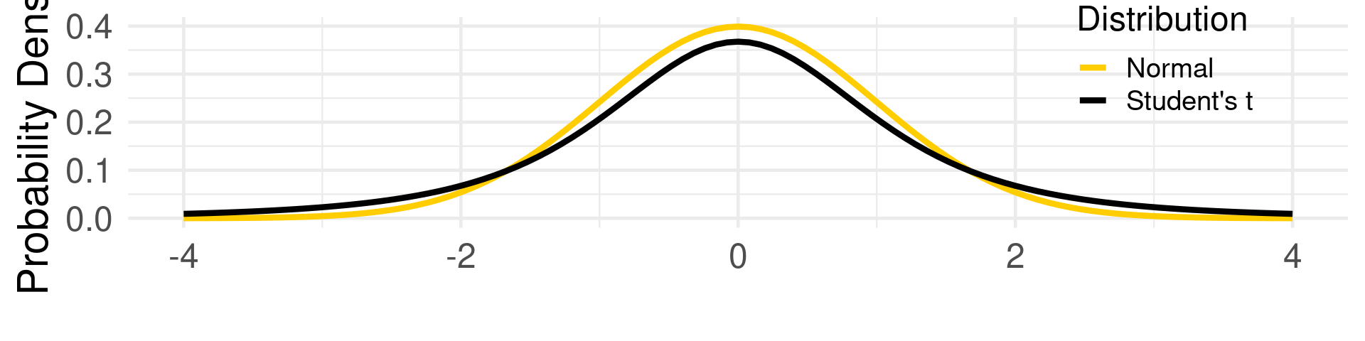
2.4 T/Student’s distribution

A researcher at Guinness had previously published a paper containing trade secrets of the Guinness brewery. The economic historian Stephen Ziliak discovered in the Guinness Archives that to prevent further disclosure of confidential information, the Guinness Board of Directors allowed its scientists to publish research on condition that they do not mention “1) beer, 2) Guinness, or 3) their own surname”.[4] To Ziliak, Gosset seems to have gotten his pen name “Student” from his 1906–1907 notebook on counting yeast cells with a haemacytometer, “The Student’s Science Notebook”[1][5] Thus his most noteworthy achievement is now called Student’s, rather than Gosset’s, t-distribution and test of statistical significance

2.5 Estimating Method

• For mean
  • σ known, \(\mu = \bar X \pm Z_{\alpha/2}\frac{\sigma}{\sqrt n}\)
  • σ unknown
    • N ≥ 100ish, then \(\bar X \pm Z_{\alpha/2}\frac{s}{\sqrt n}\);
    • N < 100ish, then \(\bar X \pm t_{\alpha/2}\frac{s}{\sqrt n}.\)

• For proportion
  • π known, \(\Pi = P \pm Z_{\alpha/2}\sqrt{\frac{\pi(1 - \pi)}{n}}\);
  • π unknown, \(\Pi = P \pm t_{\alpha/2}\sqrt{\frac{\pi(1 - \pi)}{n}}\).

• Degree of Freedom: Student’s T critical points are relative to the d.f.
  • For CI: n - 1; for regression: n - k - 1
• Procedure: Define measurement → set up α → calculate the d.f. and z/t scores → calculate the lower and upper bounds

3 Application

3.1 What can CI do

• Does an event just happen by chance?
• Is Sample A different from Sample B?

🌰 Your friend, who is the accountant for “Dr. Hu’s Amazing Team,” was asked by the organizer to help set a budget for a thank-you lunch after the team’s successful conference organization. The organizer, though unwilling to spend much, didn’t want to seem too stingy either. After calculating the average cost of lunch for a random sample of nine team members, your friend found it to be ¥29, with a ¥3 deviation, and proposed a budget of ¥31 per person. The organizer, however, criticized her, claiming “¥26 is enough” and accusing her of not understanding statistics. Is the organizer PUA your friend?

Created by DALL·E.

The ruler: Standard Normal distribution (Z-score)

3.2 PUA or not

N =9, (X̄ 29, s 3) vs. 26

PUA = Blaming someone for something they did nothing wrong.

The organizer blamed your friend for a unreasonable budget ⇒ “Unreasonable” means a guess out of the 95% CI of the sample

1. Set α = 0.05;
2. N = 9, t distribution, d.f. = 9 - 1 = 8;
3. t(α < 1 - 0.05/2) = 2.306 (qt(.975, df = 8)).
4. \(CI = 29 \pm t_{\frac{0.975}{2}}(\frac{3}{\sqrt{9}})\), i.e, [27, 31].

Created by DALL·E.

What’s the interpretation?

Inference: If we make repeated sampling from the lunch expenses, there are 95% of the samples in which the interval between 27.5 and 31.8 contains the true mean. Therefore, an estimation of 31 sounds fine. Your friend was treated unjustly.

3.3 Comparing Samples

Assuming X₁ and X₂ are i.i.d,

• σ is known, \(\mu_1 - \mu_2 = (\bar X_1 - \bar X_2) \pm Z_{\alpha/2}\sqrt{\frac{\sigma_1^2}{n_1} + \frac{\sigma_2^2}{n_2}}\).
• σ is unknown, \(\mu_1 - \mu_2 = (\bar X_1 - \bar X_2) \pm t_{\alpha/2}\sqrt{\frac{S_1^2}{n_1} + \frac{S_2^2}{n_2}}\)
  • \((\bar X_1 - \bar X_2) \pm t_{\alpha/2}S_p\sqrt{\frac{1}{n_1} + \frac{1}{n_2}}\) when the population of the samples are identical, i.e., \(\sigma_1 = \sigma_2\), where \(S_p^2 = \frac{\sum(X_1 - \bar X_1)^2 + \sum(X_2 - \bar X_2)^2}{(n_1 - 1) + (n_2 - 1)}\), d.f.: \((n_1 - 1) + (n_2 - 1)\), a.k.a., the “Difference in Means”.
• Aggregated (propotional) data: \(\Pi_1 - \Pi_2 \pm Z_{\alpha/2}\sqrt{\frac{P_1(1 - P_1)}{n_1} + \frac{P_2(1 - P_2)}{n_2}}\)

3.4 🌰

Created by DALL·E.

The “Learning R with Dr. Hu and His Friends” workshop includes two series: “R Survivor” (basic) and “R Expert” (advanced). The five “R Survivor” workshops received 932, 586, 796, 501, and 351 downloads, while the “R Expert” workshops had 771, 917, 326, 825, and 399 downloads.
Which series is more popular?

3.5 Solution

• R Survivor: 932, 586, 796, 501, and 351 downloads
• R Expert: 771, 917, 326, 825, and 399 downloads

Set α = 0.05; small N → t.

\[\begin{align} \bar X_1 =& (932 + 586 + 796 + 501 + 351)/5 = 633.2; \bar X_2 = 647.6 \\ S_p^2 =& \frac{2.151268\times 10^{5} + 2.845032\times 10^{5}}{(5 - 1) + (5 - 1)} = 6.245375\times 10^{4};\\ \mu_1 - \mu_2 =& (633.2 - 647.6) \pm 2.3646 (\sqrt{6.245375\times 10^{4}}\sqrt{1/5 + 1/5}), \\ =& -14.4 \pm 364.4763. \end{align}\]

Inference: If we make repeated sampling from the audience size of these lectures, there are 95% of the samples in which the interval between -378.8763 and 350.0763 contains the true mean. The CI covers 0. That is, the difference is no different from zero statistically.

3.6 When Not IID

IID

Observations are selected without regard to who is in the other condition, a.k.a., independent and identical distributed (IID).

Matched

Observations are matched to someone in the other condition.

3.7 Difference in Difference in Means

Independent sample

\[\mu_1 - \mu_2 = (\bar X_1 - \bar X_2) \pm t_{\alpha/2}\sqrt{\frac{S_1^2}{n_1} + \frac{S_2^2}{n_2}}\]

Matched samples

\(D = X_1 - X_2\), then \(\Delta = \bar D \pm t_{\alpha/2}\frac{S_D}{\sqrt{n}}\), where \(S_D = \sqrt{\frac{\sum(D - \bar D)^2}{n - 1}}\).

Matched proportions (Aggregate data)

\(\hat{P}_D = \frac{n_{10} - n_{01}}{n}\), then \(\Delta = \hat{P}_D \pm Z_{\alpha/2} \cdot \sqrt{\frac{n_{10} + n_{01}}{n^2}},\) where \(n\) = Number of matched pairs, \(n_{10}\) = Number of pairs where the first observation is a success and the second is not, \(n_{01}\) = Number of pairs where the first observation is a failure and the second is a success.

This formula uses the discordant pairs (\(n_{10}\) and \(n_{01}\)) to calculate the confidence interval for the difference in proportions in matched samples.

Why using a different method for matched samples? Not IID for individuals, but might for the difference

3.8 An example

Four students must achieve HSK-4 to apply to Chinese universities (fantasy). For higher-tier universities, they need even higher scores (fictional). After reviewing their initial exam results, they underwent preparatory training. The tables below show their performance in two subsequent exams.

Was the preparatory training helpful?

Student	Tim	Frank	Emily	Elise
Before	57	57	73	65
After	64	66	89	71

3.9 Solution

Student	Tim	Frank	Emily	Elise
Before	57	57	73	65
After	64	66	89	71

Set α = 0.05, \[\begin{align} D =& X_1 - X_2 \Rightarrow \bar D = \sum D / n = (7 + 9 + 16 + 6) / 4 = 9.5\\ S_D^2 =& \sum(D_i​−\bar{D})^2 = 6.25 + 0.25 + 42.25 + 12.25 = 61 / 3 \Rightarrow S_D \approx 4.51 \\ \therefore \Delta =& 9.5 \pm 3.18\times \frac{4.51}{\sqrt{4}} = 9.5 \pm 7.18 \end{align}\]

Inference: If we make repeated sampling from these students, there are 95% of the samples in which the interval between 2.32 and 16.68 contains the true mean of the difference. The CI is above 0, that is, students did get better.

3.10 Another 🌰

Gallop drew a pair of 1500 samples from the American population. In the sample of 1980, there are 52% Democrats, and 46% in the 1985 sample. Were the Democrats the same for two years, given the 95% CI?

Solution: Let α = 0.05,

\[\begin{align} \Pi_1 - \Pi_2 &= (0.46 - 0.52) \pm 1.96\sqrt{\frac{0.46 * 0.54}{1500} + \frac{0.52 * 0.48}{1500}} \\ &\approx -0.06 \pm 0.036. \end{align}\]

Inference: If we make repeated sampling from the Amercian population, there are 95% of the samples in which the interval between -0.042 and 0.03 contains the true mean. The CI contains 0. Thus, the proportion of Democrats in 1980 was not different from that in 1985 statistically at the 0.05 level.

3.11 BFF: Different Views

Bayesian

• Credible interval
• \(\theta_\text{prior-based r.v.} \in [a, b]_{fixed}\)

There are …% of the chance that the true value lies in the CI.

Some percentage of the posterior distribution lies within an particular region.

Frequentist

• Confidence interval
• \(\theta_{fixed} \in [a, b]_{r.v.}\)

There is 95% chance the CI could contain the true value (before any data is collected).

Fiducial

• (Fiducial) Conf interval
• \(\theta_{r.v.} \in [a, b]_{fixed}\)

There is 95% chance the CI could contain the true value (before any data is collected).

Fisher used it /fɪˈduʃəl/, 邓琬璐 intro to causal inference, lec 3, https://pro.yuketang.cn/v2/web/v3/playback/734415352261764864/slide/54/0

3.12 Take-home point

Appendix

Stretch

https://www.bilibili.com/video/BV1E54y1r76o/?buvid=Y045340D2FD9FA3A46419EEFE4578279ECBD&from_spmid=main.space-search.0.0&is_story_h5=false&mid=7RnjBONLRMus4FQZFBWD2g%3D%3D&p=2&plat_id=114&share_from=ugc&share_medium=iphone&share_plat=ios&share_session_id=79FE08C9-F2B1-4C18-A16C-B31179817B42&share_source=WEIXIN&share_tag=s_i&timestamp=1728732278&unique_k=skSWw7j&up_id=390316092&vd_source=f38aeefd0d38cecba9017eeee43e71c8

Meditation

松茸的世界：5分钟正念冥想-自信之心

https://www.xiaoyuzhoufm.com/episode/65b752ed0bef6c207457f51b?s=eyJ1IjogIjYwNDA1OGJiZTBmNWU3MjNiYmY3MjZiZSJ9